


1. The error of table quantity is defined as
 , (2.10)
where, α is probability; v is half price of category from last significance figure in table quantity. For example: quantity p may be 3.14. In this case v = 0.005 and
 .
.
If quantity p is 3.141 and v = 0.0005 then

and so on.
2. Error of count may occur when we measure quantity by an instrument. Typically, the error of count is half price of minimum value of instruments scale. For example a ruler has error of count vl=0.5 mm.
3. Rules of approximation: quantity x may be approximated only to two significant figures, if the first significant figure is 1 or 2. In other cases, the quantity is approximated only to one significant figure. For example: x = 0.01865, approximated quantity is 0.019; x = 0.896, approximated quantity is 0.9 and so on.
Errors of direct measurement
Errors of direct measurements are defined as
 , (2.11)
if there is one measurement (n = 1). And
 , (2.12)
if there are several measurements (n > 1).
In these equations t¥ is Student's constant, it may be defined from the table on the crossing of line with n and column with a; d is error of an instrument; v is error of count, v =d/2.
For example: the length of a body was measured three times:
| xi, mm | Dxi, mm | (Dxi)2, mm2 |
| 12.8 | -0.466 | 0.217 |
| 13.6 | 0.334 | 0.111 |
| 13.4 | 0.134 | 0.018 |
 =13.266, n=3, t=1.4, t¥=1, d=1 mm. =13.266, n=3, t=1.4, t¥=1, d=1 mm.
|
The error of this measurement will be:

The relative error is
 .
.
The final result is
x = (13.3 + 0.5) mm, a= 0.7, E = 3.6 %.
Errors of indirect measurements
Let y be indirectly measured quantity, it is defined as y = f(x1,x2,..., xn). x1,x2,..., xn is defined as the direct measurements.
1. Errors of indirect measurements are defined as
 (2.13)
if the functional dependence of investigated quantity is a polynomial.
2. Errors of indirect measurements are defined as
 (2.14)
if the functional dependence of investigated quantity, is a monomial
and we can define Dy as:  . For example:
1. If the functional dependence is  then
then

Then

2. If functional dependence is  ,
,


Then
and

The final result:  .
.
Graph presentation of the experimental results
Graph is built on the millimeter paper. In fig.2.2 you can see an example of graph.

Figure 2.2
The experimental curve is drawn through the experimental points. This curve describes the experimental data.
Control questions
1. Definition of direct and indirect measurements. Examples.
2. Definition of the most probable value of the measured quantity x.
3. What is called a relative error?
4. What is called an accidental deviation?
5. What is the equation of square mean of errors?
6. How do we define errors of instruments?
7. How do we define errors of table quantities and count errors?
8. Rules of approximation.
9. What is the equation of errors of direct measurements?
10. What is the equation of errors of indirect measurements?
Authors: S.P. Lushchin, the reader, candidate of physical and mathematical sciences.
Reviewer: S.V. Loskutov, professor, doctor of physical and mathematical sciences.
Approved by the chair of physics. Protocol № 3 from 01.12.2008.
3. ЛАБОРАТОРНА РОБОТА № 1. ВИЗНАЧЕННЯ ГУСТИНИ ТІЛ
МЕТА РОБОТИ: знайти густину металевого тіла з відомою масою, вимірюючи лінійні розміри тіла. Одержане значення густини порівняти з довідковим і визначити, з якого металу виготовлене тіло. Навчитися визначати похибки прямих і непрямих вимірювань.
ПРИЛАДИ І ЗНАРЯДДЯ: штангенциркуль, металеве тіло.
Вступ
Густиною ρ э величина, що визначається для однорідної речовини (тіла) її масою в одиниці об'єму. Тобто для однорідного тіла знаходимо
 ,
,  (3.1)
(3.1)
де m – маса тіла, V – об’єм тіла. Масу тіла в лабораторній роботі визначають як табличне значення.
Для обчислення густини тіла правильної геометричної форми проводимо вимірювання його лінійних розмірів. Далі обчислюємо об'єм за виміряними значеннями лінійних розмірів та відповідною формулою для тіла правильної геометричної форми. Нижче наведено формули об'ємів найпростіших геометричних фігур. Якщо це циліндр, то
 , (3.2)
де a – діаметр, h – висота циліндра. Для конуса
 , (3.3)
де a – діаметр основи, h – висота, π = 3,14. Для паралелепіпеда
 , (3.4)
де a, b, c три його ребра. Підставити в (3.1) відповідний об’єм і записати кінцеву робочу формулу
 .
.
Найпростішим інструментом для вимірювання лінійних розмірів є лінійка. Її найменша поділка дорівнює 1 мм. Точність вимірювання за допомогою лінійки буде дорівнювати половині ціни поділки, тобто 0,5 мм. Для вимірювань із більш високою точністю використовують штангенциркуль та мікрометр. Підвищення точності досягається завдяки використанню допоміжної шкали – ноніуса.
Штангенциркуль зображено на рисунку 3.1. Він складається з основної металевої лінійки 5 з міліметровими поділками. Па початку її розміщені нижня 6 та верхня 1 губки. Повзунок 4. нижня 7 та верхня 2 губки є одним цілим. Вони можуть переміщуватись уздовж основної лінійки 5 і фіксуватися в потрібному положенні за допомогою гвинта 3. На нижній частині повзунка 4 нанесені поділки ноніуса 8. Коли губки 6 і 7 стикаються, нуль лінійки і нуль ноніуса повинні збігатися.

1, 2 – верхні губки; 3 – фіксуючий гвинт; 4 – повзунок; 5 – лінійка;
6, 7 – нижні губки; 8 – ноніус.
Рисунок 3.1 – Штангенциркуль
Другий тип штангенциркуля зображено на рис.3.2.
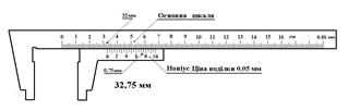
Цілі міліметри відраховуємо по основній шкалі до нульової риски шкали
ноніуса. Долі міліметра зчитуємо по шкалі ноніуса по рисці,
яка співпадає з будь-якою рискою основної шкали.
Рисунок 3.2 – Штангенциркуль.
Для того щоб виміряти довжину предмета В, його розміщують між губками 6 і 7 і закріплюють гвинтом 3. Після цього проводять відлік по лінійці і ноніусу й обчислюють довжину предмета L за формулою (9).
Для більш точного вимірювання розмірів предметів застосовуються мікрометричні гвинти з малим і точно витриманим кроком. Такі гвинти використовуються в мікрометрах. Мікрометр використовують для вимірювання зовнішніх розмірів із точністю до 0,01 мм.
Мікрометр (див. рис. 3.3) складається зі скоби 1, що має па лівому кінці нерухому п'яту 2 (перша вимірювальна поверхня), а з іншого боку – втулку 5, всередині якої встановлено мікрометричний гвинт (шпиндель) 3 з кроком 0,5 мм. Торець цього гвинта 3 і є другою вимірювальною поверхнею. На зовнішній поверхні втулки 5 проведена осьова лінія, уздовж якої нанесені поділки лінійної шкали. Верхні і нижні штрихи лінійної шкали зміщені один відносно одного на півміліметра. Цифри проставлені тільки для поділок нижньої шкали, тобто вона є звичайною міліметровою шкалою. На втулку 5 надіто барабан 6, на скошену кільцеву поверхню якого нанесено шкалу ноніуса із 50 поділками. На голівці мікрометричного гвинта 3 є пристрій 7, що забезпечує сталість тиску на вимірювальний об'єкт. Цей пристрій 7 називається тріскачкою. Для фіксування положення мікрометричного гвинта використовується стопорний гвинт 4.

1 - скоба; 2 - нерухома п'ята; 3 – торець мікрометричного гвинта;
4 - стопорний гвинт; 5 - втулка з міліметровою шкалою;
6 - барабан зі шкалою ноніуса; 7 - тріскачка.
Рисунок 3.3 – Мікрометр
Для того щоб виміряти довжину предмета, його розміщують між п'ятою 2 і торцем мікрометричного гвинта 3. Мікрометричний гвинт обертають, використовуючи тріскачку 7. При цьому мікрогвинт 3 та барабан 6 обертаються та переміщуються поступально відносно лінійної шкали на втулці 5. Обертання продовжується до зіткнення поверхонь вимірюваної деталі з вимірювальними поверхнями мікрометра 2 та 3, після чого тріскачка починає тріщати, а поступальний рух припиняється. Далі фіксують положення мікрогвинта 3 стопорним гвинтом 4. Зверніть увагу: обертати мікрометричний гвинт потрібно тільки користуючись тріскачкою 7. Інакше мікрометричний гвинт буде зірвано, мікрометр ушкоджено, вимірювання буде неправильним. Числове значення довжини вимірюваної деталі знаходять із формули:
 , (3.5)
де к – кількість поділок нижньої і верхньої лінійної шкали втулки, що відкриваються барабаном; b – відстань між сусідніми верхніми та нижніми поділками цієї шкали (0,5 мм); n – номер тієї поділки барабана, що у момент відліку збігається з осьовою лінією втулки; h – крок гвинта (0,5 мм); m – кількість всіх поділок (100) на шкалі ноніуса (барабана). Зверніть увагу: не можна починати вимірювання мікрометром, не перевіривши його початкове показання! Початкове показання мікрометра (тобто без вимірюваного тіла) повинне бути нульовим. Однак трапляються випадки, коли початкове показання мікрометра не дорівнює нулю. В такому разі потрібно визначити поправку до нульового значення (вона може бути як від'ємною, так і додатною величиною) і враховувати її під час вимірювань.
Лінійний ноніус – це невелика лінійка С (рис. 3.4) із шкалою, m поділок якої дорівнюють m-1 поділкам основної шкали масштабної лінійки А. Звідси випливає, що ціна поділки основної лінійки b та ціна поділки ноніуса а пов'язані між собою співвідношенням
 . (3.6) Величину
  називають точністю ноніуса, вона дорівнює точності вимірювання.

A - основна шкала; В - тіло, довжина якого вимірюється;
С - шкала лінійного ноніуса.
Рисунок 3.4 – Схема застосування ноніуса для вимірювання довжини тіла
Процес вимірювання полягає у такому. До нульової поділки шкали основної лінійки прикладають один кінець вимірюваною тіла В, а до іншого кінця тіла В – ноніус С. Тоді, як свідчить рисунок 3.4 шукана довжина тіла В буде дорівнювати
 , (3.7)
де розмір ΔL визначається з співвідношення (див. рис. 3.4):
 . (3.8)
Тут к – ціле число поділок масштабної лінійки; n – номер поділки ноніуса С, яка збігається з поділкою основної шкали А, Тоді з формул (3.7) і (3.8) отримуємо
 . (3.9)
Таким чином, довжина вимірюваного тіла дорівнює сумі двох величин: довжині к поділок основної шкали А, що розміщені зліва від нульової поділки ноніуса, та довжині, що дорівнює добутку точності ноніуса b/m на номер поділки ноніуса n, що збігається с поділкою основної шкали.
3.2 Вимірювання і визначення похибок
1. Висоту циліндра, конуса, або два ребра паралелепіпеда виміряти один раз.
2. Діаметр основи циліндра (конуса) або третє ребро паралелепіпеда виміряти три рази. Результати занести в таблицю.
3. Знайти середнє значення, величини діаметра, або ребра, а також відхилення від середнього значення для кожного вимірювання.
4. Розрахувати по одержаній робочій формулі густину даного тіла, підставляючи середні значення виміряних величин, і записати результат в кг/м3.
5. Визначити похибку прямих вимірювань діаметра або ребра за формулою:
 , (3.10)
де t – коефіцієнт Ст’юдента, n – число вимірювань, Dai – відхилення від середнього значення i - того вимірювання.
Таблиця 3.1
| Циліндр (Конус) | di, мм | Δdi, мм 
| (Δdi)2, мм2 | h, мм | ||||||||||||

| 
| |||||||||||||||
Таблиця 3.2
| Паралелепіпед | αi, мм | Δ α i, мм | (Δ α d) 2, мм2 | b, мм | c, мм |

| 
|
6. Півширина довірчого інтервалу величини d і α, яка вимірюється декілька разів, визначається виразом:
 , (3.11)
де d = 0,05 мм – границя основної допустимої похибки штангенциркуля.
7. Півширина довірчого інтервалу одноразових вимірювань висоти (циліндра, конуса) або ребер (паралелепіпеда) визначається виразом:
 , (3.12)
де α – довірча ймовірність, v – похибка відліку, v = 0,05 мм.
Довірчий інтервал Dm і Dp необхідно визначити як для довідкових величин. Для цього довірчу ймовірність помножають на п’ять одиниць найменшого відкинутого розряду табличного числа.
8. Відносна похибка для циліндра та конуса розраховується за формулою:
 , (3.13)
для паралелепіпеда:
 . (3.14)
9. Визначити півширину довірчого інтервалу
 . (3.15)
10. Записати кінцевий результат (висновок), застосувавши правила округлення.
11. Порівняти одержаний результат з табличними значеннями густини і визначити з якого матеріалу виготовлено зразок.
Висновок: експериментально визначена густина металевого зразка, яка дорівнює  кг/м3 =,
с довірчою імовірністю  =, відносною похибкою
  = %.
= %.
Визначено, що зразок виготовлено із ….
Контрольні запитання
1. Як Ви розумієте поняття вимірювання фізичної величини?
2. Які вимірювання називають прямими, а які непрямими?
3. В якому вигляді зазвичай записують результати вимірювань?
4. Яку інформацію мас абсолютна похибка?
5. Що такс відносна похибка?
6. Які похибки відносять до систематичних?
7. Які похибки відносять до випадкових?
8. Які похибки відносять до грубих?
9. Яку інформацію мас коефіцієнт Ст'юдепта, від яких параметрів він залежить?
10. Запишіть та поясніть формулу для абсолютної похибки випадкових похибок прямих вимірювань?
11. Запишіть та поясніть формулу для абсолютної похибки непрямих вимірювань?
12. Якою величиною характеризується точність приладів? Дайте цій величині визначення, пояснення.
13. Поясніть, скільки цифр треба залишати у записі середнього значення фізичної величини, скільки цифр треба залишати у записі абсолютної похибки?
14. Що називають густиною тіла?
15. До якого виду похибок відносять похибку штангенциркуля?
16. У чому полягає процес вимірювання за допомогою ноніуса?
17. Як побудований штангенциркуль?
18. Розкажіть, як проводити вимірювання за допомогою штангенциркуля.
19. Яку будову має мікрометр?
20. Розкажіть, як проводити вимірювання за допомогою мікрометра.
21. Для чого використовують у мікрометрі тріскачку?
22. Як знайти абсолютну похибку при вимірюванні маси?
23. Яка мета лабораторної роботи? Розкажіть про порядок виконання роботи.
24. Чому в лабораторній роботі потрібно проводити вимірювання діаметра, висоти одним і тим самим інструментом щонайменше три рази?
25. За якою формулою знаходять півширину довірчого інтервалу прямого вимірювання, виконаного декілька разів?
26. За якою формулою знаходять півширину довірчого інтервалу, якщо пряме вимірювання зроблено один раз?
27. Як знайти півширину довірчого інтервалу для табличної величини?
28. Як одержати формулу відносної похибки, виходячи з робочої формули для густини?
29. Як знайти випадкові відхилення для прямого вимірювання?
Таблиця 3.3 – Коефіцієнти Ст’юдента
| Число вимірювань, n | Довірча ймовірність, α | |||||
| 0,4 | 0,5 | 0,6 | 0,7 | 0,8 | 0,9 | |
| 0,62 | 0,82 | 1,06 | 1,4 | 1,9 | 2,5 | |
| 0,57 | 0,74 | 0,99 | 1,2 | 1,5 | 2,1 | |
| ∞ | 0,52 | 0,67 | 0,84 | 1,0 | 1,3 | 1,6 |
Таблиця 3.4 – Густина твердих тіл
| Речовина | ρ,103, кг/м3 |
| Плексиглас | 1,2 |
| Алюміній | 2,7 |
| Цинк | 7,1 |
| Залізо | 7,7÷7,9 |
| Латунь | 8,4 ÷8,7 |
| Мідь | 8,9 |
| Срібло | 10,5 |
| Вольфрам | 19,1 |
Інструкція складена доцентом кафедри фізики Корнічем В.Г.
Рецензент - доцент кафедри фізики Манько В.К.
Затверджена на засіданні кафедри фізики,
протокол № 3 від 01.12.2008 р.

