


The output of the integrating element is proportional to the integral from the input. The differential equation of this element is given by
 (3.67)
or in the operational form
 . (3.68)
The transfer function is
 , (3.69)
where T is the time constant.
The dynamic behavior of the integrating element is characterized by equation

 . (3.70)
The frequency response is described by the following expressions
 ,
,
 ,
,  ,
,  , (3.71)
 ,
,  .
.
The transient and frequency response are shown in Fig.3.20(a) and Fig.3.20(b) respectively.
.

Fig. 3.20. Transient response to a step unit input (a) and log-magnitude and phase diagram (b) for the integrating element.
Block diagram representation for integrating element is shown in Fig. 3.21.

Fig.3.21. Block diagram representation for the integrating element.
The integrating element with lag
The differential equation is given by
 (3.72)
and can be represented in the operational form as
 . (3.73)
The time response to a step unit input is written as follows
 . (3.74)
The transfer function of the integrating element with time lag is expressed by
 , (3.75)
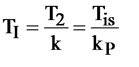
where  is the integration constant,
  .
.
The transfer function in the frequency domain is
 , (3.76)
then

 (3.77)
 (3.78)
The transient response for a step unit input and the frequency response are graphically illustrated In Fig.3.22(a) and 3.22(b) respectively.

Fig. 3.22. Transient response to a step unit input (a) and log-magnitude and phase diagram (b) for the integrating element with lag.
The diagrammatic representations of the integrating element with lag are shown in Fig. 3.23. This element can be considered as a cascade of the first order lag element with the time constant T and the integrating element with the time constant TI.
. 
Fig. 3.23. Block diagram representation of the integrating element
with time lag.
The isodromic element
The differential equation for the isodromic element (proportional plus integrating element or PI element) is given by
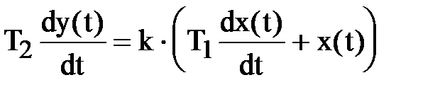 (3.79)
and can be represented in the operational form as
 . (3.80)
The transfer function is
 , (3.81)
where 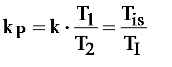 - the gain of the proportional element,
 - the isodromic constant, sec,
 - the integration constant, sec
The time response to a step unit input is described by
 . (3.82)
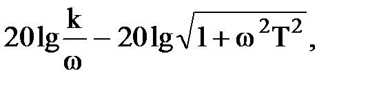
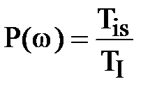
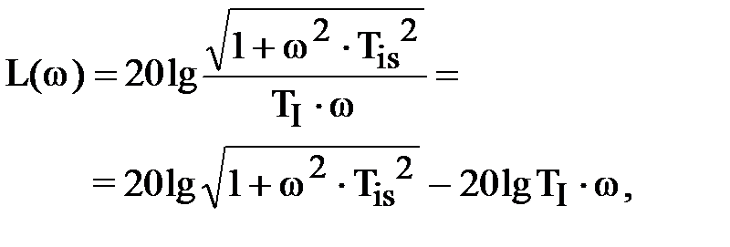
The frequency response is described as follows
 , (3.83)
 , (3.84)
 ;
;  , (3.85)
 (3.86)
 . (3.87)
The transient response to a step unit input is shown in Fig. 3.24(a). The log-magnitude and phase angle diagram is as shown in Fig. 3.24(b).
 Fig. 3.24. Transient response to a step unit input (a) and log-magnitude and phase diagram (b) for the isodromic element.
The block diagram representation of the isodromic element is shown in Fig.3.25.
 Fig. 3.25. Block diagram representation for the isodromic element.
Leading Elements

