


A general representation for a control system is shown in Fig.2.6, where y(t) is the controlled variable, x(t) is the actuating signal, and z(t) is the disturbance signal.
Table 2.1. Important Laplace transform pairs


Fig. 2.6. Generalized control system.
Generally, a control system, shown in Fig.2.6, can be described by the n-th order differential equation
 +
+  , (2.14)
where a, b, c are constants and n>m, n>k.
The general operational representation for a differential equation of order n is
 (2.15)
or in the vector form
 , (2.16)
where A(p), B(p), C(p) are polynomials in p.
The terms x(t) and z(t) are often called the forcing functions, because they force or excite the system. The output y(t) is often called the response function, because it responds to the forcing functions. Then B(p), C(p) are called the forcing operators. A(p) is called characteristic operator [4] or characteristic function [2]. The equation which results by setting the characteristic function to zero is called the characteristic equation:
 . (2.17)
The roots of the characteristic equation,  , are also called the zeros of the function A(p).
Eqs. (2.15-2.16) can be rewritten as follows
 (2.18)
 . (2.19)
Then one can define the transfer function in the operational form as the ratio of the forcing operator to the characteristic operator [4].
The operational form of the transfer function relating the output to the actuating signal can be obtained when the disturbance is assumed to be zero, z(t)=0:
 . (2.20)
The transfer function in the operational form concerning the disturbance signal can be obtained from Eq. (2.18) when the actuating signal is assumed to be zero, x(t)=0:
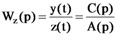 . (2.21)
Then the control system, shown in Fig.2.6, can be represented by the following equation
 . (2.22)
We can obtain the transfer function by another way using the Laplace transform [1,4].
Taking the Laplace transform of each term of Eq.(2.17) we get
 (2.23)
where  represent the initial conditions associated with each transform, L is the symbol for taking the Laplace transform.
Transforming each term of Eq.(2.17) accordingly and collecting terms yields
 (2.23)
or
 (2.24)
where  ,
,
 are the sum of all the initial conditions.
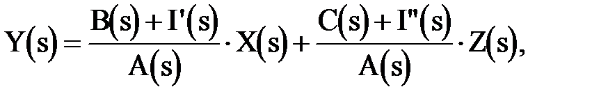
By comparison of Eqs. (2.17) and (2.24) it is to be noted that the form of the characteristic function in the s-domain, A(s), remains the same as that in the p-domain. The numerators also have the same forms with the exception that the initial conditions are added in the s-domain. Comparison of Eqs. (2.17) and (2.24) shows that, when all the initial conditions are zero, the transfer functions are obtained merely by substituting s for p, Y(s) for y(t), X(s) for x(t) and Z(s) for z(t) in the operational form of the differential equation.
Then
 (2.25)
The transfer function of a linear system in the Laplace form is defined as the ratio of the Laplace transform of the output variable to the Laplace transform of the input variable, with all initial conditions assumed to be zero:
|
|
|
 (2.26)
where A(s), B(s), C(s) are polynomials in s.
The characteristic equation may be obtained by setting the polynomial A(s) to zero
 .
.
The transfer function of a system (or element) represents the relationship describing the dynamics of the system under consideration. A transfer function may only be defined for a linear, stationary (constant parameters) system. A nonstationary system, often called a time-varying system, has one or more time-varying parameters, and the Laplace transformation may not be utilized. Furthermore, a transfer function is an input-output description of the behavior of a system. The transfer function is an important relation for control engineering. The transfer functions allow to define the transient and frequency responses of the control system and are used in block diagram models. In this text, the Heavisite operator notation is employed as an aid in obtaining the differential equations for control components and systems. We will mainly use the transfer function in the operational form. In Section 3.1 it is shown how the differential equations may be solved algebraically by the Laplace transformation technique.

