


THE GEOMETRICAL PARAMETRS OT THE 3D SURVEYS
РЕФЕРАТ
Исполнитель: ________________ М.С. Коваленко
магистрант кафедры геологии
и разведки полезных ископаемых
Рецензент: ________________ О.Н. Чалова
доцент кафедры
английского языка
Гомель, 2016
CONTENTS
| Introduction………………………………………………… | |
| 1 3D seismic surveys………………………………………… | |
| 2 The factors influence on design of 3D seismic surveys……………………………………………………………….. | |
| 3 3D data geometries……………………………………… | |
| 3.1 Data coordinates……………………………………………… | |
| 3.2 Marine-data geometries………………………………………. | |
| 3.3 Land-data geometries………………………………………... | |
| 3.3.1 Wide-azimuth geometries………………………………… | |
| Conclusion……………………………………………………… | |
| Glossary……………………………………………………….. | |
| Literature…………………………………………………….. | |
| Аннотация…………………………………………………….. |
INTRODUCTION
Seismic reflection surveys have been performed in oil exploration to delineate subsurface structure since the 1930. The early surveys (2D, single fold, continuous coverage profiling) provided large-scale structural information about the subsurface, but forced oil exploration teams to drill without a completely accurate image of the reservoir. As the use of seismic surveys became more accepted and as funds were available for research, the technique evolved until it became an effective way to view and interpret large-scale subsurface geologic structural features. The advent of the 2D, multi-fold, common-depth-point surveying techniques, along with advances in instrumentation, computers, and data processing techniques, greatly increased the resolution of seismic data and the accuracy of the subsurface images.
However, the technique still yielded little information on the physical properties of the imaged rocks, or the pore fluids within them.
It was not until the introduction of 3D reflection surveying in the 1980's that seismic images began to resolve the detailed subsurface structural and stratigraphic conditions that were missing or not discernable from previous types of data. Today potential oil reservoirs are imaged in three dimensions, which allows seismic interpreters to view the data in cross-sections along 360° of azimuth, in depth slices parallel to the ground surface, and along planes that cut arbitrarily through the data volume. Information such as faulting and fracturing, bedding plane direction, the presence of pore fluids, complex geologic structure, and detailed stratigraphy are now commonly interpreted from 3D seismic data sets.
The essence of the 3D method is a data collection followed by the processing and interpretation of a closely-spaced data volume. Because a more detailed understanding of the subsurface emerges, 3D surveys have been able to contribute significantly to the problems of field appraisal, development and production as well as to exploration. It is in these post-discovery phases that many of the successes of 3D seismic surveys have been achieved. The scope of 3D seismic for field development was first reported by Tegland.
In the late 1980s and early 1990s, the use of 3D seismic surveys for exploration has increased significantly. This started in the mid-1980s with widely-spaced 3D surveys called, for example, exploration 3D. Today, speculative 3D surveys, properly sampled and covering huge areas, are available for purchase piecemeal in mature areas like the Gulf of Mexico. This, however, is not the only use for exploration. Some companies are acquiring 3D surveys over prospects routinely, so that the vast majority of their seismic budgets are for 3D operations.
D SEISMIC SURVEYS
Seismic reflection imaging is based on the principle that acoustic energy (sound waves) will bounce, or «reflect» off the interfaces between layers within the earth’s subsurface. During a seismic reflection survey acoustic energy is imparted into the earth with a seismic source. These sources are impacted upon an aluminum strike plate ground surface to create high frequency seismic energy. After impact of the source the sound waves propagate and spread out along spherical wavefronts in all directions. The usable sound energy travels into the earth (signal), while some energy is lost into the air or along the ground surface (noise) [1].
The earth is characterized by many layers, each with different physical properties. When sound waves traveling through the earth encounter a change in the physical properties of the material in which they are traveling, they will either reflect back to the surface or penetrate deeper into the earth (where they may again be reflected at another interface). At a geologic interface some seismic energy is always transmitted while some is reflected. The acoustic impedance is a measure of how seismic energy will react when it encounters a subsurface layer. This physical property is closely associated with the density of a layer. Contrasts in acoustic impedance create seismic reflection interfaces. Subsurface reflections of seismic energy, therefore, most often occur at the interfaces between lithologic changes (a transition from sediment to rock, for example). As a result, seismic reflections make it possible to map the stratigraphy below a site.
Areas of structural deformation, such as fractures, can also be observed using seismic reflection. A fractured rock surface produces different reflections than a continuous rock surface. Acoustic energy is diffracted by fractured rock surfaces in much the same way that a visual image is distorted in a shattered mirror. Identifying diffracted energy patterns is one way in which geologic structures such as faults and fractures can be mapped using seismic reflection surveys [2].
During a seismic reflection survey high-speed digital data recording systems (seismographs) and acoustic sensors (geophones) are used to measure reflected sound waves. Compressional waves (p-waves) are a type of seismic waves. Compressional waves are so named because the wave fronts propagate through the earth mechanically; when one particle moves and compresses the next particle. The figure 1.1 (A) shows the wavefront of sound waves impinging on a geophone. The particle motion in the earth moves the geophone body, which houses a magnet within a suspended coil inside the geophone. This action produces an analog voltage signal that is proportional to the ground motion (figure 1.1(B)). The seismograph then digitizes the analog signal by breaking the signal into discrete time samples, and creates a digital level (a numeric value) for the amplitude of the signal during that time sample (figure 1.1 (C)). The data in surveys are digitized to 21-bit resolution, which means the analog geophone signal is broken into 221 or 2,097,152 levels. The analysis of the final processed wavelet (figure 1.1 (D)), which is the result of the post-survey data reduction process, and is a high resolution, distortion free representation of the subsurface [3].
Since 2D data collection occurs along a line of receivers, the resultant image represents only a section below the line. Unfortunately this method does not always produce a clear image of the geology. 2D data can often be distorted with diffractions and events produced from offline geologic structures, making accurate interpretations difficult.

Figure 1.1 – The scheme of process of transformation of a sound signal
Because seismic waves travel along expanding spherical wave fronts they have surface area. A truly representative image of the subsurface is only obtained when the entire wave field is sampled. A 3D seismic survey is more capable of accurately imaging reflected waves because it utilizes multiple points of observation. A grid of geophones and seismic source impact points are deployed along the surface of the site in a 3D survey. The result is a volume, or cube, of seismic data that was sampled from a range of different angles (azimuth) and distances (offset) (figure 1.2).

Figure 1.2 – The example of different angles (azimuth) and distances (offset)
Because oil reservoir exploration is a spatial, 3D problem, 3D seismic data collection, processing, and imaging has been advanced by all major oil companies. Today new oil reserves are very rarely located without the use of 3D imaging.
THE FACTORS influence on design
Of 3d seismic surveys
A 3D seismic acquisition survey in a complex sub-surface area is challenging. The most important geophysical factors are include: adequate fold (and hence S/N), frequency of signal available at the target, aperture (both individual shots and survey dimensions), resolution, spatial continuity of recording geometry, multiplicity of ray-paths, adequate offsets [4].
Adequate fold (and hence S/N) may be specified prior to the 3D design. This is typically based on the needs of an interpreter to identify structure times – and amplitude anomalies which may help in identifying the presence or absence of hydrocarbons. When nothing is known about the area a useful rule of thumb is to require that S/N=4. Any lower level on a final migrated stack will normally mean that the interpreter will have severe difficulties in identifying potential targets. Any higher level can be noted as an added bonus.
Once S/N of typical raw data from the area can be established, the desired fold of the survey follows as a simple calculation (formula 1):
(1) Fold = (S/N of final migrated stack / S/N of raw data)×2
Aperture, it is mean both individual shots and survey dimensions. Each shot creates a wavefield which travels into the sub-surface and is reflected upwards to be recorded at the surface. Each trace must be recorded for enough time so that reflections of interest from sub-surface points are captured – regardless of the distance from source to sub-surface point to receiver.
Also, the survey itself should be spatially large enough so that all reflections of interest are captured within the recorded area (migration aperture) and for steep dips one has to expect to add significantly to the outline of the 3D survey area. For complex areas, this step may require extensive 3D modeling.
The section shown is an “in-line” display (figure 2.1). The cross-lines showed the true three-dimensional nature of the model. Such models can be ray-traced to create synthetic 3D data volumes.
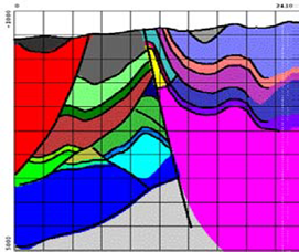
Figure 2.1 – The example of a model built for a complex sub-surface area
The complex data resulting from such ray-tracing can be created with the correct times and amplitudes. This enables an investigator to observe the effects of processing – particularly PSDM from topography.
By such means, the degree of illumination on any chosen target can be determined. In complex sub-surface areas, ray-tracing like this can establish the «visibility» or otherwise of a target for any specified 3D acquisition geometry.
Resolution is an attribute of the sub-surface. Basically it depends on the velocity of the over-burden and the frequency available at the target. Once the resolution available is calculated, the 3D designer has a choice: make the bin size equal to the horizontal resolution and therefore acquire the highest resolution survey that is possible – or make the bin size less than the available resolution and therefore discard information in the up going wavefield that describes the finer details of the sub-surface. Selecting a smaller than required bin size does not provide us with any additional information [5].
If this condition of strict spatial continuity is satisfied then the properly recorded wavefield may be used to reconstruct the subsurface reflectors to a degree of accuracy equal to the Nyquist wavelength.
This means that it does not matter how complicated the sub-surface is. From our properly sampled surface measurements we can reproduce every sub-surface wrinkle (up to Nyquist) so long as we have spatial continuity. Shots and receivers are normally laid out in some form of orthogonal grid. The sampling interval along both the shot and receiver direction determines the spatial Nyquist wavelength. Any deviation from the spacing affects the spatial continuity. Thus, for example, deleting a shot introduces a break in spatial continuity. This will manifest itself in the final migrated section as an “edge” effect which will give rise to migration noise in the area of the missing shot (diffractions).
Great attention must be given to preserving spatial continuity. Thus where obstacles are encountered, the lines (shot or receiver) must be moved smoothly around them. Any sudden changes of direction will become an «edge» with the unfortunate added migration noise.
The down going and up going wavefields can travel in very complex ways through the sub-surface. It is possible that some areas of the sub-surface may only be illuminated by portions of wavefields that have to travel great distances from source to receiver. As a result, some portions of the sub-surface may not be illuminated as well as other portions. To help with this problem the 3D designer must try to ensure that every sub-surface area of interest receives similar illumination. Extensive 3D modeling is necessary to investigate this illumination question.
Some raypaths in complex sub-surface areas can be troublesome
Physical Influences are included access problems, limitations on the design imposed by topography, limitations imposed by other environmental factors such as weather, wildlife, security of personnel and equipment, etc.
The physical influences above will clearly impose limitations on spatial continuity. The impacts of those factors should be minimized in order for us to be able to deliver the best image possible. Some migration modeling can show the designer the expected effects of severe shot and/or receiver movements.
Processing Considerations: noise removal (shot noise, multiples), removal of near surface effects (statics), analysis and application of velocity from topography (surface NMO).
The nature of offset distribution and azimuth distribution and how they change with depth is crucial in studying the noise problem. On the question of noise attenuation algorithms, the jury is still out. New processing algorithms often appear to make a substantial difference to individual shots (or receiver line components of shots). But the CMP stacks with and without the noise removal algorithm often look distressingly similar, leading to the conclusion that CMP stacking is still the best weapon in the anti-noise armory.
Delays in travel times caused by near (or even far) surface anomalies can be a source of noise. The simple perspective is that if such static delays cannot be removed they will diminish the signal content. 3D geometries differ in their ability to resolve 3D static delays. A useful rule of thumb is that the recording patch itself must be large enough to span any expected static anomaly. If a near surface static anomaly is larger than the recording patch it will be virtually impossible to remove in conventional processing.
In complex sub-surface areas, the surface topography is often highly variable. There can be very large elevation changes between shots and receivers. In such cases, the normal methods for dealing with such problems (floating datum etc.) cannot be used reliably. Instead other methods should be used which honor the different paths from shot to sub-surface and from sub-surface to receiver [6].
Successful imaging from topography – either by DMO plus post-stack migration, pre-stack time migration (PSTM) or pre-stack depth migration (PSDM).
Aperture is crucial – both the aperture recorded by single shots and that of entire surveys. And multiplicity of ray-paths is also crucial.
Some conclusions are clear. First that resolution varies throughout a survey – becoming larger near the edges and near the end of recording time (in this context, larger resolution means less ability to distinguish two adjacent sub-surface features). Second, that the size of a bin can determine resolution because of anti-alias criteria.
D DATA GEOMETRIES
Subsurface geological features of interest in hydrocarbon exploration are three dimensional in nature. Examples include salt diapirs, overthrust and folded belts, major unconformities, reefs, and deltaic sands. A two- dimensional seismic section is a cross-section of a three-dimensional seismic response. Despite the fact that a 2D section contains signal from all directions, including out-of-plane of the profile, 2D migration normally assumes that all the signal comes from the plane of the profile itself. Although out-of-plane reflections (sideswipes) usually are recognizable by the experienced seismic interpreter, the out-of-plane signal often causes 2D migrated sections to mistie. These misties are caused by inadequate imaging of the subsurface resulting from the use of 2D rather than 3D migration. On the other hand, 3D migration of 3D data provides an adequate and detailed 3D image of the subsurface, leading to a more reliable interpretation.
A typical marine 3D survey is carried out by shooting closely spaced parallel lines (line shooting). A typical land or shallow water 3D survey is done by laying out a number of receiver lines parallel to each other and placing the shotpoints in the perpendicular direction (swath shooting). Because of practical and economical considerations 3D surveys are never acquired with full regular sampling of the spatial axes. The problem of designing 3D surveys presents many more degrees of freedom than the design of 2D ones and it has no standard or unique solution [4].
The design of 3D acquisition geometries is the result of many trade-offs between data quality, logistics, and cost. Further, nominal designs are often modified to accommodate the operational obstacles encountered in the field.
Acquisition design and processing are becoming more and more connected because the characteristics of the acquisition geometry strongly influence the data processing. Understanding the principles of acquisition design is necessary to the understanding of many data processing issues. The main goal of conventional acquisition design is to obtain an adequately and regularly sampled stacked cube that can be accurately imaged by post-stack migration.
Other important design parameters are the minimum and maximum offsets. The minimum offset must be small enough to guarantee adequate coverage of shallow targets. Maximum offset must be sufficiently large to allow accurate velocity estimates that are necessary for both stacking and post-stack imaging. However, in common acquisition geometries the sampling of the offset axes may be inadequate when the data require more sophisticated pre-stack processing than simple stacking. Even the application of standard dip move out (DMO) may be problematic with some commonly used acquisition geometries. In these cases, the requirement that the midpoint axes are adequately sampled is not sufficient, because the offset and azimuth sampling play an important role as well [5].
Another important emerging issue in modern 3D survey design is subsurface illumination, as we image targets under increasingly complex overburden, and as we demand more control on the amplitudes of the images. Complex wave propagation associated with large velocity contrasts (e.g. salt or basalt bodies) may cause the data to illuminate the target only partially, even if the wavefield is sufficiently sampled at the surface. Because target illumination is strongly related to the data offset and azimuth, a careful survey design can dramatically improve the image quality. Survey-modeling tools that analyze the target illumination by ray tracing through an a priori model of the subsurface geology help to guide the design process towards successful acquisition geometries. However, the usefulness of these tools is limited by how accurately the subsurface geology and velocity model are known [3].
Although there are no preset solutions to the problem of acquisition design, there are a few acquisition schemes that are commonly used as templates to be adapted to individual surveys.
Data coordinates
In any survey, each seismic trace is characterized by the corresponding positions of its source and receiver. The coordinates of source and receiver are defined relative to an orthogonal coordinate system with x and y as the horizontal axes and z as the vertical axis. If the receivers are preferentially aligned along one direction, as they are for marine surveys and most land surveys, we will assume that the x axis is aligned with this preferential direction. In this case we will call the x axis the in-line axis and the y axis the cross-line axis. Usually the geometry space is irregularly sampled along all the axes, and often it is inadequately sampled along some or all axes, as well.
The data coordinates expressed in terms of source-receiver coordinates are often called the field coordinates, as opposed to the midpoint-offset coordinates. The midpoint-offset coordinates are defined by the following transformation of the field coordinates (formula (1) and (2)):
 (1)
(1)
 (2)
(2)
The vector m = (xm, ym) is the midpoint, and the vector h = (xh, yh) is the half-offset. Often the half-offset vector is more conveniently defined in terms of the absolute half-offset h and the source-receiver azimuth. Because the source-receiver azimuth is uniquely defined for each trace, it is often referred to as just the trace azimuth or data azimuth. This angle must be distinguished from the midpoint azimuth that is related to the geological dips in the image, as we will see in following chapters. The geometric relationships, between the field coordinate vectors (g and s) and the offset-midpoint coordinate vectors (m and h), are showed below [2].
Acquisition geometries can vary greatly according to the physical environment (e.g., land or marine), the subsurface structural complexity, and the overall goals of the survey. All the geometry templates share the common characteristic that the midpoint axes are fairly well, and often even regularly, sampled. Good sampling of the midpoint axes is necessary to accomplish the paramount goal of obtaining accurate poststack migration results.
In contrast, the sampling of the offset axes may vary according to the choice of an acquisition template.
Marine-data geometries
Modern marine data is acquired by towing several streamers behind a boat. Each streamer incorporates hundreds of hydrophones located at regular intervals. Streamers can be as long assix to eight kilometers. One or more sources of seismic energy are positioned close to the stern of the boat. Sources are usually arrays of air-guns, but experiments with marine vibroseis are yielding promising results. The boat passes over the target on multiple passes along (ideally) straight lines (called sail lines) that are equally spaced and parallel to each other. The sail-line direction is considered the in-line direction of the surveys. Currents and other factors often cause the sail-lines not to be perfectly straight; even more commonly, currents cause the streamers not to follow straight trajectories behind the boat. The lateral displacement of the streamers is often called cable feathering [5].
Another difficulty encountered in areas already developed for hydrocarbon production is that platforms, or other permanent obstacles, can be on the desired path of the boat. A technique called under-shooting is often employed to avoid gaps in the coverage of the survey just below the obstacles, which are often just above targets of interest. The data recorded by under-shooting often have a wider azimuth range and larger minimum offset than regularly recorded data; both the lack of near-offset data and the wide azimuth may cause problems during processing.
Land-data geometries
Land-data geometries vary more widely than marine ones because receiver locations are not constrained to be attached to a towed streamer. There are several possible templates that can be adopted when a land survey is designed.
One important template is cross-swath geometries. The receiver lines are crooked because of obstacles in the terrain. The sources are moved in a direction approximately orthogonal to the receiver lines; hence the name cross swath. When the source moves outside the swath covered by the receiver array, the farthest receiver line is rolled over to the side of the new shots. This acquisition configuration assures that the receiver arrays of individual shot gathers are well sampled along the receiver-line direction, but they are aliased in the orthogonal direction [5].
Conversely, common receiver gathers are well sampled along the cross-line direction, but poorly sampled along the in-line directions. Only the midpoint axes are well sampled along both directions. The offsets of a cross-swath geometry have a preferential direction aligned along the receiver lines.
Button-patch acquisition has been developed with the aim of sampling the data azimuths over the whole range between 0and 360. Wide-azimuth data are necessary to gather information on how seismic properties, such as velocity and reflectivity, vary with propagation direction.
This detailed information can be useful when the subsurface is anisotropic.
The acquisition is called «button patch» because the receivers are deployed in a checkered pattern (buttons). The ensemble of several buttons makes up a patch that is rolled along to cover contiguous areas. The receiver locations (dots) and source location (asterisk) from a shot gather recorded in Wyoming with the button-patch technique.
For the streamer geometry, only the positive half of the in-line offset component is plotted, because reciprocal traces (a trace pair with the respective source and receiver locations exchanged) provide equivalent sampling for prestack imaging operators. This comparison is only qualitative, because other factors such as propagation velocity, target depth, and signal frequency should be considered, when the sampling criteria of seismic reflections are determined [1].
However, the difference in offset coverage and trace density among the four geometries is quite dramatic. The azimuthal coverage increases as we move from streamer geometry, to parallel swath, to cross swath, and finally to the button-patch geometry.
Wide-azimuth geometries
Wide-azimuth geometries have the obvious advantage that data with different azimuths can provide useful information on the anisotropy of the subsurface, as well on the heterogeneity of the velocity field. On the other hand, if we consider the number of recorded traces as fixed, the drawback of wide-azimuth geometries is that they sample the offset plane less densely, and thus they are more subject to aliasing problems of the offset axes. This is usually not a problem if no imaging operator is applied in the prestack domain, and only trace to trace transformations, such as NMO or stacking, are applied to prestack data. However, if prestack imaging is necessary because of structural complexity (DMO) and/or strong velocity variations, the sparse sampling of the offset axes may cause artifacts in the imaging results [4].
This trade-off between the width of the azimuth coverage and data density can be avoided by either recording more traces, or by improving the methods used to prestack image wide-azimuth data.
Considerations of subsurface illumination may further complicate the trade-off between narrow and wide azimuth data. Since, under complex overburden, target illumination varies with the data azimuth, a wide-azimuth survey has «illumination holes» more uniformly distributed in the subsurface. Therefore, it has a better chance of providing at least partial information on all the geological structures than a narrow-azimuth survey has. For marine exploration, wide-azimuth OBC surveys can be used to address this problem. A practical and economical solution is to acquire two conventional narrow-azimuth data sets with the sailing directions orthogonal to each other.
To facilitate the subsequent data processing, often the order of the traces is changed according to the traces’ geometry. Sorting and binning are two common operations that reorder the traces.
Sorting is a reordering of the traces according to specific trace coordinates, called sorting in dexes. Typical sorting operations are the reordering of the data in shot gathers or receiver gathers. These sorting operations are conceptually simple because all the traces sharing the same source (receiver) location have the exact same source (receiver) coordinates. On the other hand, common-midpoint sorting is complicated by the fact that, because of irregularities in the data acquisition, traces do not share exactly the same midpoint coordinates. Therefore, common-midpoint sorting requires a prior common-midpoint binning [6].
The data are binned by superimposing a regular grid onto the midpoint plane; then all the traces that fall within each grid cell, or bin, are assigned effective midpoint-coordinates equal to the central point of the cell. The nominal bin size, that is, the length of each side of the cells, is determined by the acquisition parameters and can vary between the in-line direction and the cross-line direction. The nominal fold is equal to the number of traces that would fall in each grid if there were no irregularities in the geometry.
CONCLUSION
The primary goal of any 3D is to achieve the desired S/N at the target. In complex areas, feasibility studies are routinely done to establish suitable parameters of a 3D seismic survey and calculate an initial budget.
To ensure the best image, the best sampling method that can be used to recreate the various spatial wavelengths in X, Y and Z must be chosen. The symmetric sampling – whatever is done to shots must also be done for receivers.
Noise attenuation may be just as important as recording the signal. The «best» geometry is the one that addresses the specific local problems of improving signal at a chosen target, while identifying and reducing the various sources of noise. If the CMP stack for one geometry attenuates the noise by 6 dB, when compared to the CMP stack for another geometry, the fold has been effectively quadrupled. Today’s best geometries for noise attenuation seem to be wide azimuth slanted geometries with 18 degrees often emerging as the winning angle. The small departure from orthogonal (18 degrees instead of zero) does not dramatically affect the imaging properties.
For noise reduction (both linear, backscatter and multiples), it can be noted, that wide azimuth surveys will be better than narrow – simply because of the preponderance of long offsets. Other factors like unequal shot and receiver line spacing and slanted lines are currently under investigation.
Arrays are also making a comeback. Since 2D gave way to 3D, arrays have been largely ignored. All too often bunched phones and single holes have been the norm. Recently many acquisition geophysicists have made attempts to reduce linear and backscatter noise before it reaches the recorder.
Arrays play a crucial role in wavefield filtering and resampling to the group interval. In the absence of a geophone array, the wavefield samples collected at each surface station (group) will be aliased for all wavelengths less than the group interval. The geophone array will essentially “filter” the wavefield prior to sampling and remove this spatially aliased energy.
GLOSSARY
| A | |||
| accuracy | степень свободы от погрешности | ||
| acoustic impedance | акустическая жесткость | ||
| acoustic sensor | акустический приемник | ||
| acquisition | регистрация данных | ||
| additional correction | дополнительная поправка | ||
| advance of wave | распространение волны | ||
| air gun | пневматический излучатель упругих волн | ||
| algorithm | алгоритм | ||
| amplitude | амплитуда | ||
| analog | моделирующая система | ||
| angle | угол | ||
| anisotropy | анизотропия свойств | ||
| antialias | зеркальная частота | ||
| aperture | апертура | ||
| appraisal well | параметрическая скважина | ||
| area mapping | картирование площади | ||
| array | расположение группы сейсмоприемников | ||
| attenuation | уменьшение сигнала | ||
| azimuth | азимут | ||
| B | |||
| backscatter | рассеяние | ||
| bandwidth | диапазон частот | ||
| bin | сегмент | ||
| bottom hole | забой скважины | ||
| button | электрод микрозонда сопротивлений | ||
| C | |||
| cable | кабель | ||
| cell | ячейка | ||
| check | проверка | ||
| check shot | контрольный взрыв | ||
| coded signal | кодированный сигнал | ||
| coherent interference | когерентный шум | ||
| coherent waves | когерентные волны | ||
| common-depth-point | общая глубинная точка | ||
| common-midpoint-gather | сейсмограмма ОГТ | ||
| common-midpoint (CMP) | сейсмограмма | ||
| common-offset gather | монтаж трасс, имеющих одинаковое расстояние взрыв прибор | ||
| compression | сжатие, уплотнение | ||
| compressional wave | продольная волна | ||
| conditions | условия | ||
| conductivity | проводимость | ||
| configuration | расстановка приемников | ||
| control point spacing | шаг наблюдений | ||
| conventional processing | обработка общепринятыми методами | ||
| convergence correction | коррекция за схождение | ||
| converted wave | взрывная волна | ||
| coordinate scale | координатная сетка | ||
| correction | поправка | ||
| correction computation | вычисление поправок | ||
| coverage | дальность действия | ||
| cross-line | поперечная линия | ||
| current | ток | ||
| D | |||
| datum | уровень приведения | ||
| dB | децибел | ||
| degree | градус | ||
| delineation of structure | оконтуривание структуры | ||
| density | плотность | ||
| development | разработка | ||
| development well | эксплуатационная скважина | ||
| deviation | отклонение от вертикали | ||
| departure | отклонение от заданной величины | ||
| depth migration | глубинная миграция | ||
| depth point | глубинная точка | ||
| design | проект | ||
| desired SN | полезный сигнал | ||
| diapir | диапировая структура | ||
| diffracted wave energy | энергия отраженной волны | ||
| diffraction | дифракция | ||
| digit | однозначное число | ||
| digital section | цифровой разрез | ||
| dip angle | угол падения | ||
| dimensional parameter | пространственный параметр | ||
| direction | направление | ||
| displacement | сейсмический снос | ||
| displacement factor | компонента смещения | ||
| distance | расстояние | ||
| distribution of data | распределение данных | ||
| distinguishable velocities | различимые скорости | ||
| distortion | деформация, смещение | ||
| DMO (dip moveout) | эллиптическая развертка отражений | ||
| dot | точка | ||
| drill | буровой станок | ||
| driving point | точка возбуждения | ||
| dynamic correlation | скоростной анализ | ||
| dynamic range | динамический диапазон | ||
| E | |||
| effect | влияние | ||
| elastic waves | упругие волны | ||
| elevation | превышения | ||
| emergence | выход энергии | ||
| ensemble | выборка | ||
| estimate | приблизительный подсчет | ||
| event | волна на сейсмограмме; вступление | ||
| expanding spread | удлиненная система наблюдений | ||
| exploration | поиски и разведка месторождений | ||
| exploratory well | разведочная скважина | ||
| F | |||
| faulting | разлом | ||
| feathering | отклонение сейсмической косы от линии профиля | ||
| feature | геологический объект | ||
| field | поле | ||
| field crew | полевая партия | ||
| filter | фильтр | ||
| filtration | фильтрация | ||
| first arrivals | первые вступления волн | ||
| floating datum | переменная поверхность приведения поправок | ||
| fold | кратность | ||
| formation dip | падение пласта | ||
| folded belts | складчатая зона | ||
| fracture | трещина | ||
| frequency | частота | ||
| G | |||
| gap | интервал | ||
| gauges | регистрирующие приборы | ||
| geophone | геофон | ||
| geophysical surveys | геофизические исследования | ||
| ghost wave | волна-спутник | ||
| grid | сетка | ||
| ground | поверхность | ||
| H | |||
| head waves | головные волны | ||
| heterogeneity | неоднородность | ||
| hole | буровая скважина | ||
| hydrocarbon | углеводород | ||
| I | |||
| identify features | выделять геологическую структуру | ||
| image | мнимый источник | ||
| index | показатель, коэффициент | ||
| influence | эффект | ||
| initial data | исходные данные | ||
| in-line | вдоль линии наблюдения | ||
| interfaces | граница раздела двух сред | ||
| interference | интерференция | ||
| interpretation | интерпретация, расшифровка | ||
| K | |||
| Kirchhoff migration | миграция Киргофа | ||
| L | |||
| layer | пласт, слой | ||
| level | трасса на магнитной ленте | ||
| limitation | предел | ||
| linear system | линейная система | ||
| location | местоположение | ||
| low-velocity zone | зона малых скоростей | ||
| M | |||
| mapping limits | картируемые границы | ||
| measured amplitude | измеренные амплитуды | ||
| measurement | измерение | ||
| midpoint | серединная точка | ||
| migration | учет сейсмического сноса | ||
| mis-tie | невязка величин | ||
| mode conversion | образование обменной волны | ||
| moveout | временной сдвиг | ||
| multifold coverage | многократное перекрытие | ||
| multiple refraction | многократно преломленная волна | ||
| multiple wave | многократно отраженная волна | ||
| N | |||
| narrow-azimuth survey | узко-азимутальные исследования | ||
| NMO (normal moveout) | нормальное приращение времени | ||
| noise | помехи | ||
| notation | форма записи | ||
| numeric data | числовые данные | ||
| O | |||
| observation | наблюдения | ||
| obstacle | помехи | ||
| occurance | месторождение полезных ископаемых | ||
| offset | смещение | ||
| operation | действие, операция | ||
| organized noise | регулярные помехи | ||
| orthogonal direction | перпендикуярное направление | ||
| outline map | карта с топографической основой | ||
| output | выходной сигнал | ||
| overburden | верхняя часть разреза | ||
| overlying rocks | вышележащие породы | ||
| overthrust | надвиг | ||
| P | |||
| parallel field | однородное поле | ||
| parameter | характеристика | ||
| party | геофизическая партия | ||
| patch | большая группа сейсмоприемников | ||
| pattern | схема расстановки | ||
| peak | положительная фаза | ||
| penetration | проникновение, глубина исследования | ||
| phase | фаза | ||
| plotted section | сейсмический разрез | ||
| pore fluid | поровый флюид | ||
| positive | аномальная область, повышенных значений | ||
| post-stack migration | миграция после суммирования | ||
| preferential direction | предпочтительное направление | ||
| preliminary interpretation | предварительная интерпретация | ||
| preset parameter | установленный параметр | ||
| pre-stack migration | миграция до суммирования | ||
| pressure | давление | ||
| processing | процедура обработки | ||
| processing center | центр обработки | ||
| processing rontine | программа обработки | ||
| profile | схема расположения | ||
| profiling | профилирование | ||
| propagate | погрешность, влияющая на последующие операции | ||
| propagation | распространение | ||
| propagation constant | постоянная распространения волны | ||
| p-waves | продольная волна | ||
| Q | |||
| qualitative interpretation | качественная интерпретация | ||
| R | |||
| range | диапазон | ||
| ray path | траектория луча | ||
| ray tracing | трассировка лучей | ||
| raw data | необработанные данные | ||
| receiver | приемник | ||
| receiving point | точка приема | ||
| reciprocal time | время распространения волны во взаимных точках | ||
| recording system | регистрирующая система | ||
| recorder | записывающее устройство | ||
| reduction | приведение, поправка | ||
| reduce line | линия приведения | ||
| reef | подводная скала | ||
| reflected event | отраженная волна | ||
| reflection | отражение | ||
| reflectivity | отражательная способность | ||
| refracted waves | преломленные волны | ||
| regular grid | регулярная сеть | ||
| removal | удаление | ||
| representation | числовые данные | ||
| resampling | изменение шага кодирования | ||
| reservoir | пласт-коллектор | ||
| resolving power | разрешающая способность | ||
| resolution | разрешение | ||
| response time | время обращения сигнала | ||
| rock | порода | ||
| S | |||
| sampling | выборка дискретных данных | ||
| sampling interval | временной интервал | ||
| sand | песок | ||
| section | разрез | ||
| seismographs | сейсмическая станция | ||
| seismic data interpretation | интерпретация сейсморазведочных данных | ||
| seismogram | сейсмограмма | ||
| seismogram equipment | сейсмозаписывающая аппаратура | ||
| seismic exploration | сейсморазведка | ||
| seismic noise | сейсмические помехи | ||
| seismic profile processing | отработка сейсмического профиля | ||
| seismic vibrations | сейсмические колебания | ||
| seismic wave generation | возбуждение сейсмических волн | ||
| seismic waves | сейсмические волны | ||
| seismometer | сейсмометр | ||
| set | совокупность | ||
| scale | шкала | ||
| scattering | рассеивание | ||
| shallow water survey | геофизические исследования на мелководье | ||
| shear | сдвиг | ||
| shoot | отстрел профиля | ||
| shot | измерения, выполненные при визировании | ||
| shot noise | помехи, связанные со взрывом | ||
| shot point | точка возбуждения (колебаний) | ||
| shot recording | регистрация взрывов | ||
| side swipes | боковые отражения | ||
| signal | сигнал, несущий полезную информацию | ||
| solution | разрешение | ||
| sound wave | звуковая волна | ||
| source | источник | ||
| spacing | расстояние между приборами | ||
| span | диапазон измерения | ||
| sparse grid | редкая сетка | ||
| spatial axes | пространственные оси | ||
| static correction | статическая поправка | ||
| spread | расстановка сейсмоприемников | ||
| stack | суммарная запись | ||
| stacking | суммирование трасс | ||
| standard dip | стандартные приращения | ||
| streamer | сейсмическая коса | ||
| strike line | продольный профиль | ||
| strike plate | простирание пласта | ||
| structural complexity | сложное структурное строение | ||
| structure | сейсмическая аномалия | ||
| subsurface | недра | ||
| superposition | совмещение, суперпозиция | ||
| surface | поверхность | ||
| surface effect | влияние поверхностных изменений | ||
| surface vibration source | поверхностный источник колебаний | ||
| surface waves | поверхностные волны | ||
| survey | исследование | ||
| symmetric spacing | симметричная расстановка | ||
| synthetic data | теоритически полученные данные | ||
| s-waves | поперечные волны | ||
| T | |||
| target | сигнал | ||
| template | шаблон | ||
| terrain | рельеф местности | ||
| time of wave arrival | время вступления волны | ||
| time slices | временной срез | ||
| towing boat | судно, контролирующее сейсмокосу | ||
| trace | сейсмическая трасса | ||
| trade-off | увязка, координация | ||
| trajectory | траектория | ||
| transformation | преобразование | ||
| transition zone | переходная зона | ||
| transmit | излучатель, используемый при возбуждении импульса тока | ||
| travel time | время пробега (волны) | ||
| trough velocity | минимальная фазовая скорость | ||
| U | |||
| unconformity | несогласное стратиграфическое напластование | ||
| uniform geology | однородное геологическое строение | ||
| uphole travel time | время вертикального пробега (волны) | ||
| upward continuation | продолжение в верхнее полупространство | ||
| V | |||
| variation | отклонение | ||
| velocity | скорость распространения | ||
| velocity analysis | скоростной анализ | ||
| vibroseis data | данные метода вибросейс | ||
| vibration exciter | вибраторная установка | ||
| vibroseismics | вибросейсмика | ||
| W | |||
| wave attenuation | затухание волны | ||
| wavefield | волновое поле | ||
| waveform | форма сигнала волны | ||
| wavefront | фронт распространения волны | ||
| wavelength | длина волны | ||
| wavelet | сейсмический импульс | ||
| wave pattern | волновая картина | ||
| wave propagation line | траектория сейсмических волн | ||
| wide-azimuth-survey | широко-азимутальные исследования | ||
| well drilling | бурение скважин | ||
| width | длительность импульса | ||
| wrinkle | складка | ||
LITERATURE
1. Alistair, R. Interpretation of Three-Dimensional Seismic Data / R. Alistair. – Tulsa, Oklahoma, U.S.A: The American Association of Petroleum Geologists and the Society of Exploration Geophysicists, 2000. – 528 p.
2. Planning Land 3D Seismic Surveys / The American Association of Petroleum Geologists and the Society of Exploration Geophysicists // B. Hardage. – Tulsa, Oklahoma, U.S.A, 2000. – 205 p.
3. Biondo, L. 3D Seismic Imaging // L. Biondo. – Palo-Alto, California, U.S.A: Stanford University, 2004. – 383 p.
4. Liner, C. 3D Seismology / C. Liner // The Society of Exploration Geophysicists. – Tulsa, Oklahoma, U.S.A, 2004. – 612 p.
5. Yilmaz, Oz. Seismic data analysis. Processing, Inversion, and Interpretation of Seismic Data: in 6 volumes // Oz. Yilmaz. – Tulsa, Oklahoma, U.S.A: The Society of Exploration Geophysicists, 2001. – Vol. 2. – 1053 p.
6. Satinder, C. Seismic attributes for prospect identification and reservoir characterization / C. Satinder // The Society of Exploration Geophysicists. – Tulsa, Oklahoma, U.S.A, 2007. – 448 p.
АННОТАЦИЯ
Внедрение в практику геологоразведочных работ на поисково-разведочном этапе объемной или трехмерной сейсморазведки 3D явилось отражением характерных тенденций в развитии современных технологий и использовании их в геофизических исследованиях. Это обусловлено объективными причинами, такими как необход

