


(COMPUTER VARIANT)
The aim: investigation of atomic spectrum; define the Plank’s constant.
Instrumentation and appliances: computer.
Course of the work
1. Examine the spectrums of the radiation of helium, hydrogen and mercury.
2. Examine the spectrum of the Sun’s radiation.
Pay attention to yellow, light-green and blue line of mercury on long-wave part of helium spectrum. Define from what levels 4 lines of the spectrum of the hydrogen appear. Have in mind that for all line of the visible spectrum transition is realized on the second quantum level.
3. Measure the lengths of the waves of the spectrum of the hydrogen radiation.
Do the measurements with a virtual rules. The rules moves up and down at snub by mouse on field from the side of spectrum.
4. Define the frequencies for these line.
On measured length of the waves calculate the frequencies of these four lines.
5. Define the Plank’s constant.
On formulas of Born’ theories calculate a Plank’s constant for these four lines, but the results do average.
6. Do the conclusion.
In conclusion pay attention to the lengths of the radiation and absorptions lines. Also pay attention to spectrum regularities and possibility on spectrum’s lookout to define the Plank’s constant.
Authors: Serpetsky B.A., the reader, candidate of physical and mathematical sciences.
Reviewer: Loskutov S.V., professor, doctor of physical and mathematical sciences.
Газовий лазер
Газовий лазер (г. л.) - лазер з газоподібним активним середовищем. Трубка з активним газом вміщується в оптичний резонатор, що в простому випадку складається з двох паралельних дзеркал, одне з яких є напівпрозорим.
Випущена в якому-небудь місці трубки світлова хвиля при розповсюдженні її через газ посилюється за рахунок актів вимушеного випускання, що породжують лавину фотонів. Дійшовши до напівпрозорого дзеркала, хвиля частково проходить через нього. Ця частина світлової енергії випромінюється зовні. Інша ж частина відбивається від дзеркала і дає початок новій лавині фотонів. Всі фотони ідентичні по частоті, фазі і напряму розповсюдження. Завдяки цьому випромінювання лазера може мати надзвичайно велику монохроматичність, потужність і різку спрямованість.
Перший г. л. був створений в США в 1960 А. Джаваном. Сучасні лазери працюють в дуже широкому діапазоні довжин хвиль - від ультрафіолетового випромінювання до далекого інфрачервоного випромінювання - як в імпульсному, так і в безперервному режимі. У табл. приведені деякі дані про найбільш поширені Р. л. безперервної дії.
З г. л., що працюють тільки в імпульсному режимі, найбільший інтерес представляють лазери ультрафіолетового діапазону на іонах Ne ( = 0,2358 мкм і = 0,3328 мкм) і на молекулах N2 ( = 0,3371 мкм). Азотний лазер володіє великою імпульсною потужністю.
У випромінюванні г. л. найвиразніше виявляються характерні властивості лазерного випромінювання - висока спрямованість і монохроматичність. Істотною гідністю є їх здатність працювати в безперервному режимі. Застосування нових методів збудження (див. нижчий) і перехід до вищого тиску газу можуть різко збільшити потужність г. л. За допомогою г. л. можливе подальше освоєння далекого інфрачервоного діапазону, діапазонів ультрафіолетового і рентгенівського випромінювань. Відкриваються нові області застосування г. л., наприклад в космічних дослідженнях.
Щодо особливості газів як лазерних матеріалів, то в порівнянні з твердими тілами і рідинами гази мають істотно меншу щільністю і вищу однорідність. Тому світловий промінь в газі практично не спотворюється, не розсівається і не зазнає втрат енергії. У таких лазерах порівняно просто порушити тільки один тип електромагнітних хвиль (одну моду). В результаті спрямованість лазерного випромінювання різко збільшується, досягаючи межі, обумовленого дифракцією світла. Розходімость світлового променя г. л. в області видимого світла складає 10-5 - 10-4 радіан, а в інфрачервоній області 10-4 - 10-3 радіан.
На відміну від твердих тіл і рідин, складові газ частинки (атоми, молекули або іони) взаємодіють один з одним тільки при зіткненнях в процесі теплового руху. Ця взаємодія слабо впливає на розташування рівнів енергії частинок. Тому енергетичний спектр газу відповідає рівням енергії окремих частинок. Спектральні лінії, відповідні переходам частинок з одного рівня енергії на іншій, в газі розширені трохи. Вузькість спектральних ліній в газі приводить до того, що в лінію потрапляє мало мод резонатора.
Оскільки газ практично не впливає на розповсюдження випромінювання в резонаторі, стабільність частоти випромінювання г. л. залежить головним чином від нерухомості дзеркал і всієї конструкції резонатора. Це приводить до надзвичайно високої стабільності частоти випромінювання г. л. Частота, що випромінювання г. л. відтворюється з точністю до 10-11, а відносна стабільність частоти
 (22.1)
Мала щільність газів перешкоджає отриманню високої концентрації збуджених частинок. Тому густина енергії, що генерується, у г. л. істотно нижче, ніж у твердо тільних лазерів.
Активним середовищем г. л. є сукупність збуджених частинок газу (атомів, молекул, іонів), що мають інверсну населеність енергетичних рівнів. Це означає, що число частинок, що «населяють» вищі рівні енергії, більше, ніж число частинок, що знаходяться на нижчих енергетичних рівнях. У звичайних умовах теплової рівноваги має місце зворотна картина - населеність нижчих рівнів більша, ніж вищих. У разі інверсії населеностей акти вимушеного випромінювання фотонів з енергією h  = Ев - Ен, супроводжуючі вимушений перехід частинок з верхнього рівня Ев на нижній Ен, переважають над актами поглинання цих фотонів. В результаті цього активний газ може генерувати електромагнітне випромінювання частоти
 (22.2)
або з довжиною хвилі
 (22.3)
Одна з особливостей газу (або суміші газів) - різноманіття фізичних процесів, що приводять до його збудження і створення в нім інверсії населеностей. Збудження активного середовища випромінюванням газорозрядних ламп, що знайшло широке застосування в твердо тільних і рідинних лазерах, мало ефективно для отримання інверсії населеностей в г. л., оскільки гази володіють вузькими лініями поглинання, а лампи випромінюють світло в широкому інтервалі довжин хвиль. В результаті може бути використана тільки нікчемна частина потужності джерела накачування (ККД малий). У переважній більшості г.л. інверсія населеностей створюється в електричному розряді (газорозрядні лазери). Електрони, що утворюються в розряді, при зіткненнях з частинками газу (електронний удар) порушують їх, переводячи на вищі рівні енергії. Якщо час життя частинок на верхньому рівні енергії більший, ніж на нижньому, то в газі створюється стійка інверсія населеностей. Збудження атомів і молекул електронним ударом є найбільш розробленим методом отримання інверсії населеностей в газах. Метод електронного удару застосовний для збудження Р. л. як у безперервному, так і в імпульсному режимах.
Збудження електронним ударом вдало поєднується з іншим механізмом збудження - передачею енергії, необхідної для збудження частинок одного сорту від частинок іншого сорту при не пружних зіткненнях (резонансна передача збудження). Така передача вельми ефективна при збігу рівнів енергії у частинок різного сорту (рис.12.1).
У цих випадках створення активного середовища відбувається в два етапи: спочатку електрони порушують частинки допоміжного газу, потім ці частинки в процесі не пружних зіткнень з частинками робочого газу передають їм енергію. В результаті цього населяється верхній лазерний рівень. Щоб добре накопичувалася енергія, верхній рівень енергії допоміжного газу повинен володіти великим власним часом життя. Саме по такій схемі здійснюється інверсія населеностей в гелій-неоновому лазері.
Гелій-неоновий лазер (А. Джаван, США, 1960). У гелій-неоновому лазері робочою речовиною є нейтральні атоми неону Ne. Атоми гелію Не служать для передачі енергії збудження. У електричному розряді частина атомів Ne переходить з основного рівня Е1 на збуджений верхній рівень енергії E3. Але в чистому Ne час життя на рівні E3 малий, атоми швидко «зіскакують» з нього на рівні E1 і E2, що перешкоджає створенню достатньо високої інверсії населеностей для пари рівнів E2 і E3. Домішка Не істотно міняє ситуацію. Перший збуджений рівень Не співпадає з верхнім рівнем E3 неону. Тому при зіткненні збуджених електронним ударом атомів Не з не збудженими атомами NT (з енергією E1) відбувається передача збудження, в результаті якої атоми NT будуть збуджені, а атоми Не повернуться в основний стан. При достатньо великій кількості атомів Не можна добитися переважного заселення рівня неону. Цьому ж сприяє спустошення рівня E2 неону, що відбувається при зіткненнях атомів із стінками газорозрядної трубки. Для ефективного спустошення рівня E2 діаметр трубки повинен бути достатньо малий. Проте малий діаметр трубки обмежує кількість NT і, отже, потужність генерації, Оптимальним, з погляду максимальної потужності генерації, є діаметр близько 7 мм. Т. о., в результаті спеціального підбору кількостей (парціального тиску (Див. Парціальний тиск)) NT і Не і при правильному виборі діаметру газорозрядної трубки встановлюється стаціонарна інверсія населеностей рівнів енергії E2 і E3 неону.
Рівні мають складну структуру, тобто складаються з безлічі підрівнів. В результаті гелій-неоновий лазер може працювати на 30 довжинах хвиль в області видимого світла і інфрачервоного випромінювання. Дзеркала оптичного резонатора мають багатошарові діелектричні покриття. Це дозволяє створити необхідний коефіцієнт віддзеркалення для заданої довжини хвилі і порушити тим самим в г. л. генерацію на необхідній частоті.
Основний конструктивний елемент гелій-неонового лазера - газорозрядна трубка (зазвичай з кварцу). Тиск газу в розряді 1 мм. рт. ст., причому кількість Не звичайно в 10 разів більше, ніж NT. На рис. 2 приведена конструкція гелій-неонового лазера, розроблена для застосування у відкритому космосі. Розрядна трубка з внутрішнім діаметром 1,5 мм з корундової кераміки поміщена між напівпрозорим дзеркалом і призмою, що відображає, змонтованими на жорсткій берилієвій трубі (циліндрі). Розряд здійснюється на постійному струмі (8 мА, 1000 в) в двох секціях (кожна завдовжки 127 мм) із загальним центральним катодом. Холодний оксидно танталовий катод (діаметром 48 мм і довжиною 51 мм) роздільний на 2 половини діелектричною прокладкою, що забезпечує однорідніший розподіл струму по поверхні катода. Вакуумні сильфони з неіржавіючої сталі, що є анодами, утворюють рухоме з'єднання кожної трубки з утримувачами дзеркала і призми. Кожух завершений з лівого кінця вихідним вікном. Лазер розрахований на роботу в космосі протягом 10 000 ч.
Потужність випромінювання гелій-неонових лазерів може досягати десятих доль Вт, ККД не перевищує 0,01%, але висока монохроматичність і спрямованість випромінювання, простота в обігу і надійність конструкції зумовили їх широке застосування. Червоний гелій-неоновий лазер ( = 0,6328 мкм) використовується при юстіровочних і нівелювальних роботах (шахтні роботи, кораблебудування, будівництво великих споруд). Гелій-неоновий лазер широко застосовується в оптичному зв'язку і локації, в голографії (Див. Голографія) і в квантових гіроскопах (Див. Квантовий генератор).
Лазер на вуглекислому газі (До. Пател, США, Ф. Легей, Н. Легей-соммер, Франція, 1964). Молекули, на відміну від атомів, мають не тільки електронні, але і т.з. коливальні рівні енергії, обумовлені коливаннями атомів, складових молекулу, щодо положень рівноваги (див. Молекула). Переходи між коливальними рівнями енергії відповідають інфрачервоному випромінюванню. Лазери, в яких використовуються ці переходи, називаються молекулярними. З числа молекулярних лазерів особливо цікавий лазер, в якому використовуються коливальні рівні молекули СО2, між якими створюється інверсія населеностей (СО2-лазер).
У газорозрядних СО2 - лазерах інверсія населеностей також досягається збудженням молекул електронним ударом і резонансною передачею збудження. Для передачі енергії збудження служать молекули азоту N2, що порушуються, у свою чергу, електронним ударом. Зазвичай в умовах тліючого розряду близько 90% молекул азоту переходить в збуджений стан, час життя якого дуже великий. Молекулярний азот добре акумулює енергію збудження і легко передає її молекулам СО2 в процесі не пружних зіткнень. Висока інверсія населеностей досягається при додаванні в розрядну суміш Не, який, по-перше, полегшує умови виникнення розряду і, по-друге, через свою високу теплопровідність охолоджує розряд і сприяє спустошенню нижніх лазерних рівнів молекули СО2. Ефективне збудження СО2-лазеров може бути досягнуте хімічними або газодинамічними методами.
Тонка структура коливальних рівнів молекули СО2 дозволяє змінювати довжину хвилі (перебудовувати лазер) скачками через 30-50 Ггц в інтервалі довжин хвиль від 9,4 до 10,6 мкм.
СО2-лазери володіють високою потужністю (найбільша потужність лазерного випромінювання в безперервному режимі) і високим ккд. При збудженні молекул СО2 електронним ударом і довжині газорозрядної труби 200 м СО2-лазер випромінює потужність 9 кВт. Існують компактні конструкції з вихідною потужністю в 1 кВт. Окрім високої вихідної потужності, СО2-лазери володіють великими ККД, такими, що досягає 15-20% (можливе досягнення ККД 40%). СО2-лазери можуть принципово ефективно працювати і в імпульсному режимі. Перераховані особливості Co2-лазеров обумовлюють різноманіття їх застосування: технологічні процеси (різання, зварка), локація і зв'язок (атмосфера прозора для хвиль з л = 10 мкм), фізичні дослідження, пов'язані з отриманням і вивченням високотемпературної плазми (Див. Плазма) (висока потужність випромінювання), дослідження матеріалів і так далі
Газорозрядні трубки СО2-лазеров мають діаметр від 2 до 10 см, довжина їх може бути дуже великою (мал. 3). Зазвичай застосовуються секційні (модульні) конструкції із струмом розряду до декількох а при напрузі до 10 кВ на секцію. Т. до. потужність СО2-лазеров безперервної дії досягає дуже високих значень, серйозною проблемою є виготовлення достатньо довговічних дзеркал хорошої оптичної якості. Застосовуються покриті золотом сапфірові або металеві дзеркала. Виведення випромінювання часто проводиться через отвори в дзеркалах. Як напівпрозорі вихідні дзеркала застосовуються пластини з високоомного германію, арсеніду галію і тому подібне
У електричному розряді СО2-лазеров мають місце небажані ефекти, що руйнують інверсію населеностей, - розігрівання газу і дисоціація його молекул. Для їх усунення газова суміш безперервно «проганяється» через розрядні труби лазерів. Так відбувається оновлення активного середовища. Для отримання великих потужностей (декілька кВт) в безперервному режимі газ проганяють через трубку з великою швидкістю і розряд відбувається в надзвуковому потоці. Для того, щоб уникнути втрат дорогого Не, газова суміш циркулює по замкнутому контуру. Збудження електронним ударом проводиться або в резонаторі, або безпосередньо перед надходженням суміші в резонатор. У кращих приладах практично всі молекули СО2, що влітають в резонатор, вже збуджені і за час прольоту через резонатор віддають енергію збудження у вигляді кванта випромінювання.
Іонні лазери (У. Бріджес, США, 1964). У іонних лазерах інверсія населеностей створюється між електронними рівнями енергії іонізованих атомів інертних газів і пари металів. Інверсія населеностей досягається вибором пари рівнів, для якої нижній лазерний рівень володіє меншим, а верхній - великим часом життя. Необхідність створення великої кількості іонів приводить до того, що щільність струму газового розряду в іонних лазерах досягає десятків тисяч а/см2 Електричний розряд здійснюється в тонких капілярах діаметром до 5 мм. При великій щільності струму газ захоплюється струмом від анода до катода. Для компенсації цього ефекту анодна і катодна області розрядної трубки з'єднуються додатковою довгою трубкою малого діаметру, що забезпечує зворотний рух газу.
Зважаючи на високу щільність струму для виготовлення газорозрядних трубок іонних лазерів застосовуються металокерамічні конструкції або трубки з берилієвої кераміки, що володіють високою теплопровідністю. ККД іонних лазерів не перевищує 0,01%. В області видимого світла порівняно високою потужністю в безперервному режимі володіють аргонові лазери. Аргоновий іонний лазер генерує випромінювання з = 0,5145 мкм (зелений промінь) потужністю до декількох десятків Вт. Він застосовується в технології обробки твердих матеріалів, при фізичних дослідженнях, в оптичних лініях зв'язку, при оптичній локації штучних супутників Землі.
Іонний лазер на суміші іонів аргону і криптону володіє здатністю перебудовуватися по довжині хвилі (зміною дзеркал) у всьому видимому діапазоні. Він випромінює потужність до 0,1 Вт на хвилях 0,4880 мкм (синій), 0,5145 мкм (зелений), 0,5682 мкм (жовтий) і 0,6471 мкм (червоний промінь).
Вельми перспективний лазер на парах кадмію, що працює в безперервному режимі в синій (0,4416 мкм) і ультрафіолетовою (0,3250 мкм) областях спектру і що володіє високою монохроматичністю. Пара Cd утворюється у випарнику, розташованому біля анода (мал. 4). Вони сильно розбавлені Не. Рівномірний розподіл Cd в газорозрядній трубці і підбір його концентрації досягаються захопленням пари Cd іонами Не від анода до катода. Щільність пари Cd визначається температурою підігрівача. У охолоджувачі біля катода Cd конденсується. Трубка діаметром 2,5 мм і завдовжки 140 см при тиску Не 4,5 мм рт.ст. ст.ст., температурі підігрівача 250 °С, струмі розряду 0,12 а і напрузі 4 кВ дозволяє отримати потужність 0,1 Вт в сині і 0,004 Вт в ультрафіолетовій областях спектру. Кадмієвий лазер застосовується в оптичних дослідженнях (див. Нелінійна оптика), океанографії, а також фотобіології і фотохімії.
Газодинамічні лазери (В. К. Конюхов і А. М. Прохоров, СРСР, 1966). Характерною особливістю газів є можливість створення швидких потоків газових мас. Якщо заздалегідь сильно нагрітий газ раптово розширюється, наприклад при протіканні з надзвуковою швидкістю через сопло, то його температура різко падає. При раптовому зниженні температури молекулярного газу коливальні рівні енергії молекул можуть виявитися збудженими (газодинамічне збудження). Існує Со2-лазер з газодинамічним збудженням. При газодинамічному збудженні теплова енергія безпосередньо перетвориться в енергію електромагнітного випромінювання. Потужність випромінювання газодинамічних лазерів, що працюють в безперервному режимі, досягає 100 кВт.
Хімічні лазери. Інверсія населеностей в деяких газах може бути створена в результаті хімічних реакцій, при; яких утворюються збуджені атоми, радикали або молекули. Газове середовище зручне для хімічного збудження, оскільки реагуючі речовини легко і швидко перемішуються і легко транспортуються. Хімічні лазери цікаві тим, що в них відбувається пряме перетворення хімічної енергії в енергію електромагнітного випромінювання. Прикладом хімічного збудження може служити збудження при ланцюговій реакції з'єднання фтору з дейтерієм, в результаті якої виходить збуджений дейтерид фтору DF, передавальний надалі енергію свого збудження молекулам СО2. Видалення продуктів реакції забезпечує безперервний характер роботи цих лазерів.
До хімічних лазерів примикають г. л., у яких інверсія населеностей досягається за допомогою реакцій фотодиссоціації (розпаду молекул під дією світла). Це реакції, що швидко відбуваються і в ході яких виникають збуджені радикали або атоми. Існує лазер на фотодиссоціації молекули Cfзi (С. Р. Раутіан, І. І. Собельман, СРСР). Дисоціація відбувається під дією випромінювання ксенонової лампи-спалаху. Уламком реакції є збуджений атомарний іон I+.
Порівняльна таблиця різних видів лазерів
| Лазер | Довжина хвилі, мкм | Потужність, Вт |
| Кадмієвий | 0,3250 | декілька тисячних доль |
| Кадмієвий | 0,4416 | десяті долі |
| Аргоновий | 0,4880 | одиниці |
| Аргоновий | 0,5145 | десятки |
| Криптоновий | 0,5682 | одиниці |
| | Гелій-неоновий | 0,6328 | десяті долі |
| Гелій-неоновий | 1,1523 | соті долі |
| Ксеноновий | 2,0261 | соті долі |
| Гелій-неоновий | 3,3912 | соті долі |
| СО-лазер | 5,6-5,9 | сотні |
| СО2-лазер | 9,4-10,6 | дес. тисяч |
| Лазер на молекулах HCN | тисячні долі |
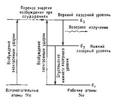
Рисунок 22.1 Схема рівнів енергії допоміжних і робочих частинок газорозрядного лазера.

Рисунок 22.2 Поперечний перетин конструкції гелій-неонового лазера для космічних досліджень.

Рисунок 22.3 Схематичне зображення кадмієвого лазера: 1 - дзеркала; 2 - вікна для виходу випромінювання; 3 - катод (зліва) і анод (справа); 4 - випарник кадмію; 5 - конденсатор пари кадмію; 6 - газорозрядна трубка.
Геrлій-неоrновий лаrзер - невеликий лазер, часто використовуваний в лабораторних дослідах і оптиці. Має робочу довжину хвилі 632,8 нм, розташовану в червоній частині видимого спектру.
Робочим тілом гелій-неонового лазера служить, як зрозуміло з назви, суміш двох газів - гелію і неону в пропорції 5:1, розташованою в скляній колбі під низьким тиском (звичайне близько 300 Па). Енергія накачування подається від двох електричних розрядників з напругою близько 1000 вольт, розташованих в торцях колби. Резонатор такого лазера зазвичай складається з двох дзеркал - повністю непрозорого з одного боку колби і другого, проникного через себе близько 1 % падаючого випромінювання на вихідній стороні пристрою.
Гелій-неоновиє лазери компактні, типовий розмір резонатора - від 15 см до 0,5 м, їх вихідна потужність варіюється від 1 до 100 мвт.
Принцип дії
У газовому розряді в суміші гелію і неону утворюються збуджені атоми обох елементів. При цьому виявляється, що енергії метастабільного рівня гелію 1S0 і випромінювального рівня неону 2p55s 2 [1/2] виявляються приблизно рівними - 20.616 і 20.661 ев відповідно. Передача збудження між двома цими станами відбувається в наступному процесі:
He* + Ne + Де = He + Ne*
і її ефективність виявляється дуже великою (де (*) показує збуджений стан, а Де - відмінність енергетичних рівнів двох атомів.) ті, що не дістають 0.05 ев беруться з кінетичної енергії руху атомів. Заселеність рівня неону 2p55s 2 [1/2] зростає і в певний момент стає більш ніж у рівня 2p53p 2, що пролягає нижче [3/2]. Наступає інверсія заселеності рівнів - середовище стає здібним до лазерної генерації.
Під час переходу атома неону із стану 2p55s 2 [1/2] в стан 2p53p 2 [3/2] випускається випромінювання з довжиною хвилі 632.816 нм. Стан 2p53p 2 [3/2] атоми неону також є випромінювальними з малим часом життя і тому це стан швидко девозбуждаєтся в систему рівнів 2p53s а потім і в основний стан 2p6 - або за рахунок випускання резонансного випромінювання (випромінюючі рівні системи 2p53s), або за рахунок зіткнення із стінками (метастабільні рівні системи 2p53s).
Крім того при правильному виборі дзеркал резонатора можна отримати лазерну генерацію і на інших довжинах хвиль: той же рівень 2p55s 2 [1/2] може перейти на 2p54p 2 [1/2] з випромінюванням фотона з довжиною хвилі 3.39 мкм, а рівень 2p54s 2 [3/2], що виникає при зіткненні з іншим метастабільним рівнем гелію, може перейти на 2p53p 2 [3/2], іспустя при цьому фотон з довжиною хвилі 1.15 мкм. Також можливо отримати лазерне випромінювання на довжинах хвиль 543,5 нм (зелений), 594 нм (жовтий) або 612 нм (оранжевий).
Смуга пропускання, в якій зберігається ефект посилення випромінювання робочим тілом лазера, досить вузька, і складає близько 1,5 Ггц, що пояснюється наявністю доплерівського зсуву. Ця властивість робить гелій-неоновиє лазери хорошими джерелами випромінювання для використання в голографії, спектроскопії, а також в пристроях прочитування штріх-кодов.
Література
1. Квантова електроніка, М., 1969; Беннет В.,
2. Газові лазери, пер. з англ., М., 1964;
3. Блум А., Газові лазери, «Тр. інституту інженерів по електроніці і радіоелектроніці», 1966, т. 54, F 10;
4. Пател До., Могутні лазери на двоокиси вуглецю, «Успіхи фізичних наук», 1969, т. 97, в. 4;
5. Аллен Л., Джонс Д., Основи фізики газових лазерів, пер. з англ., М., 1970.
Laser
In 1953 Basov, Prohorov (Soviet physicists) and independently from them Townes (American physicist) created first molecular generators called lasers which worked in the range of centimeter waves. In 1960 Meiman (USA) created analogical device working in the optical range (Light Amplification by Simulated Emission of Radiation) – laser or optical quantum generator.
There are solids, gas, semiconductor and liquid lasers accordingly to the type of medium. Laser consists of: active medium, system of pumping, optical resonator. The scheme of laser is shown in Fig. 13.1.The active medium amplifies light. System of pumping realizes tran

Figure 23.1
sition of medium to the state with population inversion. For the selection of direction of laser radiation optical resonator is used. For example, a pair of parallel mirrors facing each other being on the common optical axis between which optical medium exists. One of the mirrors is semitransparent through which numerically amplified flux of photons laser radiation escapes.
Let us consider the work of He-Ne laser (Fig.13.2).

Figure 23.2
Population inversion of levels is realized trough electrical discharge: electrons formed in discharge excite atoms of He at collision that transfer to the state 3.
At the collisions of excited He atoms with Ne atoms excitation of them occurs and they pass to higher level situated near respective He level. Passing of Ne atoms from the high level 3 to the lower level 2 causes laser radiation of λ = 0,6328 μ. Laser radiation is characterized by:
1) High time and space coherence.
2) rigid monochromatism ( );
);
3) the high power of radiation;
4) very small angular discrepancy of the beam.
The use of laser is very wide: machining of materials, research of plasma, in the measuring devices, in medicine.
Література
1. Ландcберг Г. С. Оптика. – М.: Наука, 1976.
2. Сивухин Д. В. Общий курс физики. – т. 4. – М.: Наука, 1980.
3. Савельев И. В. Курс общей физики.– т. 2. – М.: Наука, 1982.
4. Яворський В. М., Детлаф А. А. Курс загальної фізики т. 3.
5. Фріш С. Е., Тімофеєв А. В. Курс загальної фізики т. 3.
6. Квантова електроніка, М., 1969; Беннет В.,
7. Газові лазери, пер. з англ., М., 1964;
8. Аллен Л., Джонс Д., Основи фізики газових лазерів, пер. з англ., М., 1970.

