


ON MODEL
A purpose of the work is to obtain equipotential lines and lines of force of an electrostatic field and determine its intensity.
Instrumentation and appliances: a power source; a potentiometer; a panel with electrodes and conducting paper; a probe; an oscilloscope.
Theoretical part
An electrostatic field is created by immobile charges and determined in each point of space by the force acting on a test charge.
The main characteristic of an electrostatic field is the intensity
 , (11.1)
where  is the force acting on a point charge q placed into the point under consideration.
An energetic characteristic of an electrostatic field is the electrostatic potential U. It is measured by the work that is performed by an electric force when a unit positive charge is shifted from this point to the infinity.
When a charge shifts from arbitrary point 1 to arbitrary point 2, the work performed is independent of a trajectory and due to a difference of potentials:
 . (11.2)
Potential is a function of coordinates  . If a potential distribution is known, an intensity can be found being
 , (11.3)
where operator grad in the right side is called the gradient. It acts on scalar function of coordinates  by the rule
 . (11.4)
 are unit vectors along axis x, y and z respectively.
An electrostatic field can be represented with equipotential surfaces (equipotential lines in two-dimensional case). The equipotential surface (line) is a locus of points with equal potential.
To represent an electrostatic field lines of force (lines of intensity) can be also used. The line of force is a line with tangent at each point coinciding with vector of intensity. Constructing lines of force, one can use their properties:
a) lines of force start from positive charges and finish at negative ones (or disperse in infinity);
b) crossing equipotential surfaces (lines), lines of force are directed perpendicularly to them;
c) lines of force come out (or come in) perpendicularly to electrodes since charged metallic surfaces are equipotential;
d) lines of force are concentrated in the places where intensity is higher;
e) lines of force are directed down in potential.
There is an analogy between of an electrostatic potential distribution in a homogeneous dielectric medium and a potential distribution in a homogeneous conductor with an electric current. It can be explained by the fact that both cases are described by the same equation which doesn't include any parameter of a medium
 . (11.5)
This equation can be applied to a dielectric as well as to a conductor. It is possible to study an electrostatic field in a dielectric medium by measuring a distribution of potential in a conductor although this potential distribution is of different origin.
Experimental part
A potential distribution in a thin conducting layer is used in this work as a two-dimensional model for an electrostatic field. To measure potential, a bridge is used (fig. 11.1). Two metal electrodes A and B are pressed to the sheet of paper with a conducting layer. Voltage U o = 6.3 V passes from the source to electrodes and lower terminals of the potentiometer. Probe P is connected to the sliding contact S through terminals of vertical deflection of the oscilloscope (input Y).
The oscilloscope is used in the work as an indicator of presence of a potential difference. When the probe touches the surface of the conducting paper we observe a signal on oscilloscope screen (as a vertical intercept, height of which is proportional to a potential difference between a point of contact and sliding contact S). If potential at the point of contact is equal to one at sliding contact, a dot is seen on the screen.

Figure 11.1
At the beginning two or three sheets of paper with outlines of electrodes in the position taking place during the work have to be inserted under electrodes and conducting paper.
We consider potential of the electrode A to be equal to zero U А = 0. Then U В = 6.3 V (only an amplitude value of the potential is taken into account). To obtain an equipotential curve for some value  , first it is needed to place sliding contact S in the appointed position (fig. 11.2)
 . (11.6)
Then it is necessary to move probe P along the conducting layer in direction of decreasing oscilloscope signal and stop the probe when the signal becomes zero. Potential at the stop point is equal to Ui. In order to fix position of this point pierce all the sheets by top of the probe.
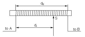
Figure 11.2
Near this point, another one with potential Ui has to be found and fixed. In such a way, moving from point to point, one can obtain the sequence of pinholes by which the equipotential curve can be drawn when the paper sheets are put out.
1. Obtain equipotential curves varying value of potential from 0 to 6.3 V with a step of 0.9 V. Take into consideration that outlines of electrodes are equipotential curves corresponding to potential values 0 and 6.3 V.
2. Build up a system of lines of force (not less than 7 in number).
3. Determine value and direction of an intensity at the points indicated by teacher. Value of intensity can be found by using the approximate formula
 , (11.7)
where Un and Un+1 are potentials of two equipotential curves nearest to the point being considered; D is length of the shortest intercept joining these curves and coming through the point.
4. Estimate an error in location of equipotential curves
 , (11.8)
where k (in V/a scale graduation) is position of the voltage divider at the Y input of the oscilloscope.

