If you scroll through a lot of data in a worksheet, you’ll probably lose sight of the column headings as they disappear off the top of your “page”. This can make life really difficult – imagine trying to check a student’s result for tutorial 8 in row 183 of the worksheet! And it’s even more difficult if the student’s name in column A has scrolled off the left edge of the window.
The Freeze Panes feature allows you to specify particular rows and columns that will always remain visible as you scroll through the worksheet. And it’s easy to do!
Select a cell immediately below the rows that you want to remain visible, and immediately to the right of the columns that you want to remain visible. For example, if you want to be able to see Rows1 and 2, and column A, then you would click on cell B3.

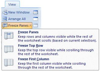
On the View tab, click Freeze Panes, and select the first option.

If Freeze Panes has already been applied, then the ribbon option automatically changes to Unfreeze Panes.
Formulas
Formulas are the key to Excel’s amazing power and versatility! By using a formula, you can find the answer to virtually any calculation you can think of! In this section I’m going to explain how to construct a formula, and give you some guidelines to ensure that your formulas work correctly.
Creating a formula
Rule number one: a formula always starts with an equals sign (“=”). This lets Excel know that it’s going to have to work something out.
In the body of the formula, you’re going to tell Excel what you want it to calculate. You can use all the standard maths operations, like addition and multiplication, and you can include numbers, cell references, or built in functions (which are covered in the next section of this manual).
For example, suppose you have a retail business. You buy stock at cost price, and add a 25% markup to calculate your selling price. VAT must be added to that at 14%. You give a 5% discount to long-standing customers who pay their accounts promptly. Let’s look at how formulas can make the calculations simple for you:

• In column A, the Stock Item labels have just been typed in.
• In column B, the Cost Price values have just been typed in.
• In column C, I’ve used a formula. Cell C2 contains “=B2 * 25%”. This works out 25% of the value in cell B2 (cost price), and displays the result in cell C2 (markup).
• In column D, I’ve used a formula. Cell D2 contains “=B2 + C2”. This adds the values in cells B2 (cost price) and C2 (markup), and displays the result in cell D2 (retail price).
• In column E, I’ve used a formula. Cell E2 contains “=D2 * 14%”. This works out 14% of the value in cell D2 (retail price), and displays the result in cell E2 (VAT).
• In column F, I’ve used a formula. Perhaps by now you can work it our for yourself? Cell F2 contains “=D2 + E2”. This adds the values in cells D2 (retail price) and E2 (VAT), and displays the result in cell F2 (selling price).
• In column G, I’ve used a formula. Cell G2 contains “=F2 * 95%”. This works out 95% of the value in cell F2 (selling price), and displays the result in cell G2 (discounted price).
And the great thing about using formulas in Excel, is that you can copy them just as you do values. So once you’ve entered all the formulas in row 2 and checked that they are correct, you just need to
1. Select the cells in row 2 that contain your formulas (cells C2 to G2).
2. Move the cursor over the fill handle in the bottom right corner of the selected cells. It will change shape to a black cross.
3. Hold down the mouse button and drag the selected cells over rows 3 to 5. The values in cells C3 to G5 are automatically calculated for you! How cool is that?


