


Ћабораторна робота є4
“ема: Ђ¬≥дновленн€ зображеньї
¬иконав:
ст. гр. ‘“ћ5
–оманчук —.
ѕерев≥рила:
“умська ќ.¬.
Ћьв≥в - 2016
ћета роботи: досл≥дити способи генеруванн€ випадкового шуму з заданими параметрами та ефективн≥сть р≥зних метод≥в в≥дновленн€ спотворених зображень.
‘ункц≥њ системи MATLAB:
1. imnoise - моделюванн€ спотворенн€ зображенн€ шумом.
¬ основному дана функц≥€ призначена дл€ створенн€ тестових зображень, використовуваних при вибор≥ метод≥в ф≥льтрац≥њ шуму, проте може застосовуватис€ ≥ дл€ доданн€ фотореал≥стичност≥ штучно синтезованим зображенн€м.
2. imnoise2 - генеруванн€ випадкового шуму.
Ќа в≥дм≥ну в≥д imnoise, функц≥€ imnoise2 породжуЇ шумову матрицю R розм≥ру MxN, €ка не нормуЇтьс€. ≤нша значна в≥дм≥нн≥сть в≥д функц≥њ imnoise пол€гаЇ в тому, що виходом imnoise служить зашумлене зображенн€, a imnoise2 породжуЇ т≥льки шумову матрицю. ористувач повинен сам задавати бажан≥ параметри шуму. Ўумова матриц€, що генеруЇтьс€ за методом Ђс≥ль ≥ перецьї, приймаЇ три можливих значенн€: 0 - це Ђперецьї, 1 - Ђс≥льї, а 0.5 в≥дпов≥даЇ в≥дсутност≥ шуму.
3. imnoise3 - моделюванн€ пер≥одичного шуму.
4. roipoly - ≥нтерактивний виб≥р област≥ Ђ≥нтересуї (ROI).
÷€ функц≥€ виводить зображенн€ S у в≥кно ≥ оч≥куЇ в≥д користувача визначенн€ област≥ ≥нтересу. якщо при виконанн≥ функц≥њ параметр S опущений, то зображенн€ беретьс€ з поточного в≥кна. »нтересующа€ область зображенн€ повинна бути обведена пол≥гоном, вершини €кого задаютьс€ одноразовим натисканн€м л≥воњ клав≥ш≥ миш≥. ѕопередню задану вершину можна видалити, €кщо натиснути на клав≥ш≥ Backspace або Delete. Ќатисканн€ на праву кнопку миш≥ або подв≥йне клацанн€ л≥вою клав≥шею задаЇ останню вершину пол≥гону. “акож завершити процес завданн€ вершин без вказ≥вки останньоњ можна натисканн€м на клав≥шу Enter.
5. histroi - побудова г≥стограми област≥ ROI.
6. statmoments - обчисленн€ середнього значенн€ ≥ центральних статистичних момент≥в.
7. checkerboard - побудова макетного зображенн€ шаховоњ дошки.
8. fspecial - формуванн€ просторового ф≥льтра (маски).
ѕовертаЇ маску h з умовного двовим≥рного л≥н≥йного ф≥льтра, що задаЇтьс€ р€дком type. ћаска h призначена дл€ передач≥ у функц≥њ filter2 або conv2, що виконують двовим≥рну л≥н≥йну ф≥льтрац≥ю. «алежно в≥д типу ф≥льтра дл€ нього можуть бути визначен≥ один або два додатков≥ параметри –1, –2.
9. imfilter - виконанн€ ф≥льтрац≥њ зображенн€.
‘≥льтруЇ багатовим≥рний масив A багатовим≥рним ф≥льтром H. ћасив A повинен бути числовим масивом будь-€кого формату ≥ розм≥рност≥. –езультуючий масив B маЇ ту ж розм≥рн≥сть ≥ формат представленн€ даних, що ≥ масив A.
ожен елемент результуючого масиву B обчислюЇтьс€ з використанн€м чисел подвоЇноњ точност≥ плаваючою крапкою. якщо A Ї масив ц≥лих чисел, тод≥ елементи результуючого масиву, що перевищують допустимий д≥апазон, ус≥каютьс€ ≥ округл€ютьс€.
10. deconvwnr - застосуванн€ ≥нверсноњ та в≥неровськоњ ф≥льтрац≥њ.
¬≥дновлюЇ зображенн€ I, €ке було з≥псовано з функц≥Їю прот€жност≥ точки PSF ≥ можливим доповненн€м шуму. јлгоритм оптим≥зуЇтьс€ з погл€ду найменшоњ середньоквадратичноњ помилки м≥ж обчислюваним ≥ вих≥дним зображенн€ми ≥ використовуЇ матрицю корел€ц≥њ та шуму. ѕри в≥дсутност≥ шумовий складовоњ, ф≥льтр ¬≥нера перетворюЇтьс€ в ≥деальний ≥нверсний ф≥льтр.
|
|
|
’≥д роботи:
«адача ви€вленн€ спотворенн€ зображенн€ виконуЇтьс€ за зображенн€ми, на €к≥ накладаЇтьс€ шум.
ѕор€док опрацюванн€ зображень:
1) ћоделюванн€ зображенн€, спотвореного адитивним шумом.
a) √енеруванн€ шуму з обраними параметрами.
b) Ќакладанн€ шуму на зображенн€.
2) ќц≥нка параметр≥в шуму.
a) ¬иб≥р област≥ Ђ≥нтересуї.
b) ѕобудова г≥стограми по област≥ Ђ≥нтересуї.
c) ¬изначенн€ статистичних параметр≥в за г≥стограмою област≥ Ђ≥нтересуї.
d) ѕобудова теоретичних г≥стограм розпод≥л≥в функц≥й шуму за визначеними статистичними параметрами.
e) ѕор≥вн€нн€ г≥стограми област≥ Ђ≥нтересуї з теоретичними г≥стограмами.
f) ¬изначенн€ характеру шуму.
3) ¬≥дновленн€ зображенн€(усуненн€ шуму).
a) ¬иб≥р функц≥й дл€ усуненн€ шуму.
b) ”суненн€ шуму на зображенн≥ за вибраною функц≥Їю.
c) ѕобудова к≥нцевоњ г≥стограми за областю Ђ≥нтересуї на в≥дф≥льтрованому зображенн≥.
d) ѕор≥вн€нн€ г≥стограм.
—потворенн€ зображенн€ адитивним шумом виконуЇмо в наступному пор€дку:
Ј «авантажуЇмо зображенн€, використовуючи оператор imread та виводимо його на екран з допомогою оператора imshow.
Ј ¬иконуЇмо ≥нтерактивний виб≥р на зображенн≥ област≥ однор≥дного с≥рого тону Ц област≥ Ђ≥нтересуї (ROI) за допомогою функц≥њ roipoly. (ѕрактично це така область, в €к≥й розпод≥л €скравостей створений головним чином шумом.) ¬ нашому випадку ми будемо моделювати зашумлене зображенн€.
Ј ЅудуЇмо г≥стограму област≥ ≥нтересу, використовуючи функц≥ю histroi.
Ј «а допомогою функц≥њ imnoise накладаЇмо шум √аусса.
Ј ЅудуЇмо г≥стограму зашумленого зображенн€.
ƒал≥ виконуЇмо оц≥нку параметр≥в зашумленого зображенн€:
Ј ¬икористовуючи функц≥ю statmoments визначаЇмо середнЇ значенн€ та дисперс≥ю розпод≥лу шуму.
Ј «а визначеними параметрами за допомогою функц≥њ imnoise2 будуЇмо теоретичну г≥стограму.
¬≥дновленн€ спотвореного зображенн€ за допомогою ф≥льтр≥в виконуЇмо у такому пор€дку:
Ј ¬≥дновлюЇмо зображенн€ за допомогою нел≥н≥йного середнього геометричного ф≥льтра та будуЇмо його г≥стограму.
Ј —потворюЇмо зображенн€ шумом Ђс≥ль та перецьї ≥ в≥дновлюЇмо його за допомогою мед≥анного ф≥льтра.
ƒл€ моделюванн€ пер≥одичного шуму використовуЇмо такий програмний код:
clc % очищенн€ командного в≥кна
clear % очищен€ робочоњ област≥
f=imread(' D:\ћаткад\–оманчук\Cyfrova obrobka \vazon.tif');% вв≥д зашумленого зображенн€
figure (1)
imshow(f); %вив≥д зображенн€ на екран
title ('«ашумлене зображенн€');
xlabel(Romanchyk., ‘“ћ5');
% ¬в≥д заданоњ б≥нарноњ маски
B=imread(' maskbinary.tif');
figure (2)
imshow(B);
title ('Ѕ≥нарна маска ¬');
%вим≥рюванн€ координат вершин б≥нарноњ маски
% - б≥н≥рна маска, с - коорд. стовпц≥в, r - коорд. р€дк≥в
% в режим≥ step вим≥рюЇмо координати вершин б≥нарноњ маски
[K, c, r]=roipoly(B);
figure (3)
imshow(K);
title ('Ѕ≥нарна маска K');
xlabel(Romanchyk., ‘“ћ5');
% √≥стограма област≥ ROI на зображенн≥ t п≥д K
p=imhist(f(K));
%figure (4)
%imshow(K);
% р - г≥стограма, npix - к≥льк≥сть п≥ксел≥в ROI
[p,npix]=histroi(f,c,r);
|
|
|
npix
figure (4)
bar(p, 1);
title ('√≥стограма област≥ ROI на зображенн≥ t п≥д K');
xlabel(Romanchyk., ‘“ћ5');
% v(1)- середнЇ значенн€, v(2) - дисперс≥€
[v, unv]=statmoments(p,2);
var=sqrt(v(2))*256;
ms=v(1)*256;
% √енеруванн€ √аусового шуму
X=imnoise2('gaussian', npix, 1, ms, var);
figure (5)
hist(X, 130);
axis([0 300 0 140])
title (['“еоретична г≥стограма, середн.=', num2str(ms, 3), ' скв=', num2str(var, 3)]);
xlabel(Romanchyk., ‘“ћ5');
ќтриман≥ результати:
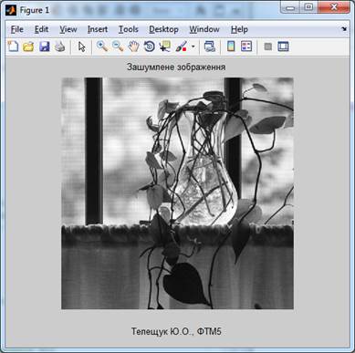
–ис.1.«ашумлене зображенн€
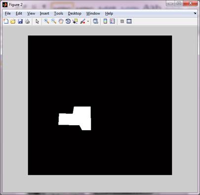
–ис.2.
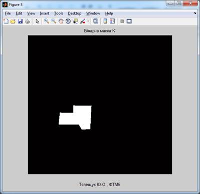
–ис.3.Ѕ≥нарна маска K

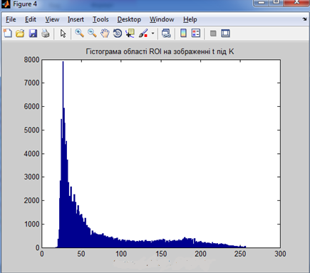
–ис.4.√≥стограма област≥ ROI
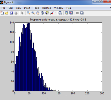
–ис.5.“еоретична г≥стограма
ƒл€ моделюванн€ зашумленого зображенн€ створюЇмо ћ-файл, у €кий записуЇмо наступний програмний код:
clc % очищенн€ командного в≥кна
clear % очищен€ робочоњ област≥
% ћоделюванн€ зашумленого зображенн€
f=imread('Tracy.tif');% вв≥д зображенн€
figure (1)
imshow(f); %вив≥д зображенн€ на екран
title ('ѕочаткове зображенн€');
xlabel(Romanchyk., ‘“ћ5');
t=imnoise(f, 'gaussian',0, 0.01);
figure (2)
imshow(t);
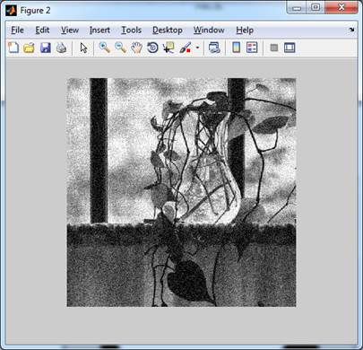
title ('«ашумлене зображенн€');
xlabel(Romanchyk., ‘“ћ5');
% «апис на диск
imwrite(t, 'Shum_Tracy.tif')
%¬иб≥р област≥ ≥нтересу
B=roipoly(t);
figure (3)
imshow(B);
title ('Ѕ≥нарна маска ¬');
xlabel(Romanchyk., ‘“ћ5');
%¬им≥рюванн€ координат вершин б≥нарноњ маски
% - б≥н≥рна маска, с - коорд. стовпц≥в, r - коорд. р€дк≥в
% в режим≥ step вим≥рюЇмо координати вершин б≥нарноњ маски
[K, c, r]=roipoly(B);
figure (3)
imshow(K);
title ('Ѕ≥нарна маска K');
xlabel(Romanchyk., ‘“ћ5');
% √≥стограма област≥ ROI на зображенн≥ t п≥д K
p=imhist(t(K));
%figure (4)
%imshow(K);
% р - г≥стограма, npix - к≥льк≥сть п≥ксел≥в ROI
[p,npix]=histroi(f,c,r);
npix
figure (4)
bar(p, 1);
title ('√≥стограма област≥ ROI на зображенн≥ t п≥д K');
% v(1)- середнЇ значенн€, v(2) - дисперс≥€
[v, unv]=statmoments(p,2);
var=sqrt(v(2))*256;
ms=v(1)*256;
% √енеруванн€ √аусового шуму
X=imnoise2('gaussian', npix, 1, ms, var);
figure (5)
hist(X, 130);
axis([0 300 0 140])
title (['“еоретична г≥стограма, середн.=', num2str(ms, 3), ' скв=', num2str(var, 3)]);
ќтриман≥ результати:
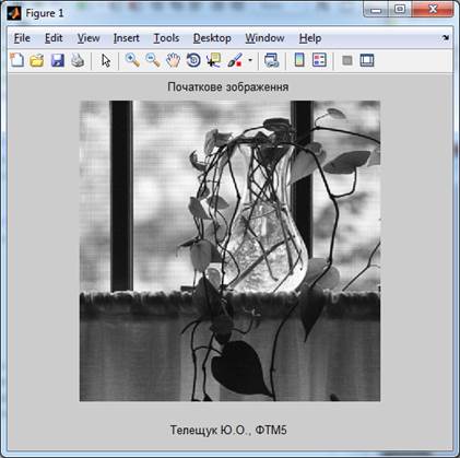
–ис.6.¬их≥дне зображенн€
–ис.7.Ѕ≥нарна маска √ауса
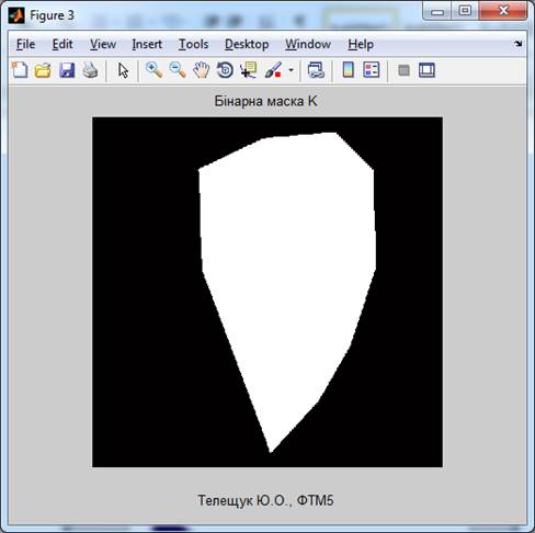
–ис.8.Ѕ≥нарана маска
–ис.9.
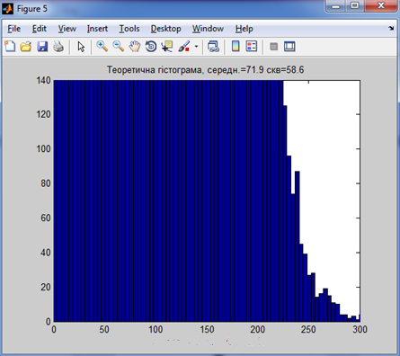
–ис.10.“еоретична г≥стограма
ƒл€ в≥дновленн€ зображенн€ створюЇмо новий ћ-файл з наступним програмним кодом:
clc % очищенн€ командного в≥кна
clear % очищен€ робочоњ област≥
% ¬≥дновленн€ зображенн€
g=imread('Shum_Tracy.tif');% вв≥д зашумленого зображенн€
figure (1)
imshow(g); %вив≥д зображенн€ на екран
title ('«ашумлене зображенн€');
xlabel(Romanchyk., ‘“ћ5');
% јрифметичний середн≥й ф≥льтр
w=fspecial('average', [3,3]); % ‘ормуванн€ маски 3*3
gr=imfilter(g, w, 'replicate'); % поширенн€ зображенн€ з використанн€м опц≥њ replicate
figure (2)
imshow(gr, []);
title ('¬≥дновлене зображенн€, арифметичний середн≥й ф≥льтр');
% √еометричний середн≥й ф≥льтр
f=im2double(g);
f1=padarray(f, [5,5], 'replicate');
f=colfilt(f1, [3,3], 'sliding', @gmean);
f1=im2uint8(f);
figure (3)
imshow(f1);
title ('¬≥дновлене зображенн€, геометричний середн≥й ф≥льтр');
% ћед≥анний ф≥льтр
f=imread('Tracy.tif');% вв≥д зображенн€
figure (4)
imshow(f);
fn=imnoise(f, 'salt & pepper');
figure (5)
imshow(fn);
title ('—потворене зображен€, с≥ль ≥ перець');
Q=medfilt2(fn, [3,3], 'symmetric');
figure (6)
imshow(Q);
title ('¬≥дновлене зображенн€, ћед≥анний ф≥льтр');
% ‘≥льтр м≥н≥муму
f2=ordfilt2(g, 1, ones(3*3));
figure (7)
imshow(f2);
title ('¬≥дновлене зображенн€, ‘≥льтр м≥н≥муму');
% ‘≥льтр максимуму
f3=ordfilt2(g, 3*3, ones(3*3));
figure (8)
imshow(f3);
title ('¬≥дновлене зображенн€, ‘≥льтр максимуму');
ќтриман≥ результати:
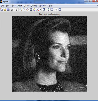
–ис.11.«ашумлене зображенн€
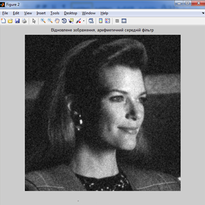
–ис.12.јрефметичний середн≥й ф≥льтр
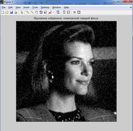
–ис.13. √еометричнийй середн≥й ф≥льтр
|
|
|
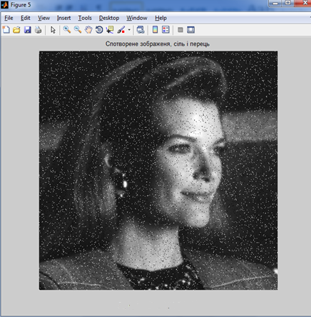
–ис.14.—творене зображенн€,с≥ль ≥ перець
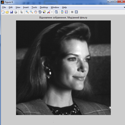
–ис.15.ћед≥анний ф≥льтр
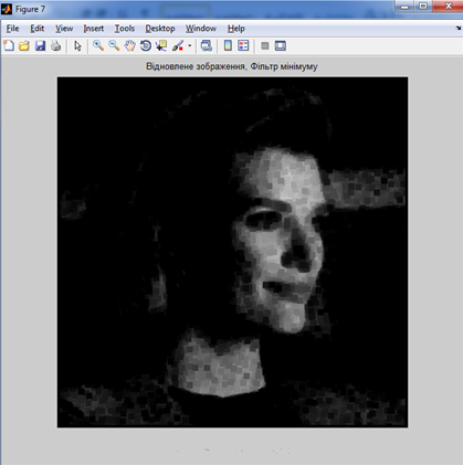
–ис.16.‘≥льтр м≥н≥муму
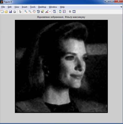
–ис.17.‘≥льтр максимуму
¬исновок: €к бачимо з наведених г≥стограм, дл€ усуненн€ гауссового шуму найкращ≥ результати даЇ середн≥й геометричний ф≥льтр. ћед≥анний ф≥льтр даЇ результати т≥льки, €кщо зображенн€ спотворене шумом типу Ђс≥ль ≥ перецьї.
¬≥дновленн€ змазаного ≥ зашумленого зображенн€
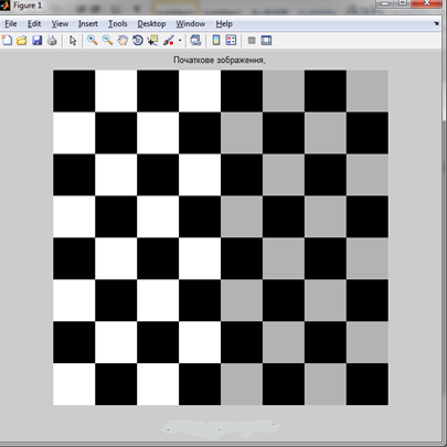
a) √енеруванн€ макетного зображенн€.
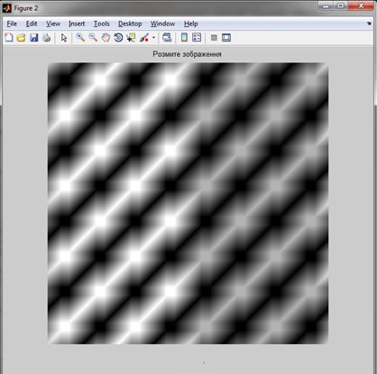
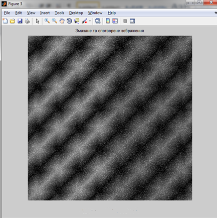
b) √енеруванн€ змазаного та спотвореного зображенн€.
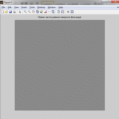
c) ¬≥дновленн€ змазаного та спотвореного зображенн€.
—творюЇмо ћ-файл, у €кий вводимо в≥дпов≥дний програмний код:
%√енеруванн€ змазаного та спотвореного зображенн€
clc
clear
%f=checkerboard(8);
f1= imread('Tracy.tif');
f=im2double(f1);
PSF= fspecial ('motion', 70, 45);
figure (1);
imshow(f);
title ('ѕочаткове зображенн€,')
%√енеруЇмо змазане зображенн€, спотворюЇмо його √аусовим шумом та виведемо
%його на екран за допомогою наступного тексту програми:
g=imfilter(f, PSF, 'circular');
figure(2);
imshow(g);
noise=imnoise(zeros(size(f)), 'gaussian', 0,0.1);
gb=g+noise;
figure(3);
imshow(gb,[]);
title ('«мазане та спотворене зображенн€');
% fr1 - результат пр€мого застосуванн€ ≥нверсноњ ф≥льтрац≥њ
fr1=deconvwnr(gb,PSF);
% обчисленн€ числа R
Sn=abs(fft2(noise)).^2; % noise power spectrum
nA=sum(Sn(:))/prod(size(noise)); % noise avarage power
Sf=abs(fft2(f)).^2; % image power spectrum
fA=sum(Sf(:))/prod(size(noise)); % image avarage power
R=nA/fA;
% ¬≥дновленн€ зображенн€ з R
fr2=deconvwnr(gb,PSF,R);
% в≥дображенн€
figure(4), imshow(fr1, [])% пр€ме застосуванн€ ≥нверсноњ ф≥льтрац≥њ
title ('ѕр€ме застосуванн€ ≥нверсноњ ф≥льтрац≥њ');
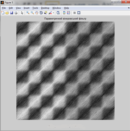
figure(5), imshow(fr2, [])% параметричний в≥неровський ф≥льтр
title ('ѕараметричний в≥неровський ф≥льтр');
% ¬икористан€ автокорел€ц≥йних функц≥й
NCORR=fftshift(real(ifft2(Sn)));
ICORR=fftshift(real(ifft2(Sf)));
fr3=deconvwnr(gb,PSF,NCORR,ICORR);
% в≥дображенн€
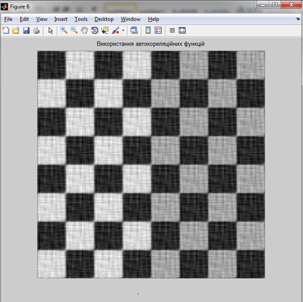
figure(6), imshow(fr3, [])% використанн€ автокорел€ц≥йноњ функц≥њ
title ('¬икористанн€ автокорел€ц≥йних функц≥й');
ќтриман≥ результати:
–ис.18.
–ис.19.
–ис.20.
–ис.21.
–ис.22.
–ис.23.
¬исновок: дл€ в≥дновленн€ змазаного ≥ спотвореного зображенн€ використовуЇмо ≥нверсну ф≥льтрац≥ю, параметричний в≥неровський ф≥льтр ≥ автокорел€ц≥йну функц≥ю. Ќайкращ≥ результати даЇ автокорел€ц≥йна функц≥€.

