Magnetic field distribution along

AN AXIS OF A CIRCULAR CURRENT

A purpose of the work is to test relation between magnitude of a magnetic intensity and a distance along an axis of a circular current.

Instrumentation and appliances: a panel with two coils and scale; an audio-signal generator; a milliammeter.

Theoretical part

The main characteristic of a magnetic field in a medium is the magnetic induction which is determined by the force acting on an element of a conductor with a current:

, (13.1)

where I is a current; is the vector which magnitude is equal to length of a conductor section and it’s direction coincides with a current direction. The boldface multiplication sign denotes the vector product.

Currents of any origin are sources of a magnetic field. Closed microscopic currents related to, for example, motion of electrons in atoms are always presented in a medium. Hence the total magnetic field in a medium is the sum of the field produced by macroscopic currents in conductors and one produced by microscopic currents in a magnetized medium (a magnetic) :

, (13.2)

where H/m. is called the intensity of a magnetic field, is the magnetic polarization.

For a homogeneous isotropic medium (nonferromagnetic), relation between magnetic polarization and intensity is considered to be linear:

. (13.3)

The proportionality coefficient is called the magnetic susceptibility. After substitution of (13.3) into (13.2), we obtain the relationship between induction and intensity

, (13.4)

where is called the magnetic permeability of the medium. In contrast to the dielectric permeability, the magnetic permeability can be either much or less than 1. Typical values of susceptibility for nonferromagnetic substances are 0.38×10^-⁶ (air), -26×10^-6 (silver), 300×10^-6 (platinum).

Magnetic intensity at an arbitrary point is determined by a current distribution in conductors. If currents flow along wires, intensity at distances much more than a transverse size of the wires can be found by using the Biot-Savart-Laplace formula

. (13.5)

In this formula, identifies position of the point where intensity has to be found; is the radius-vector of the wire element (this vector is defined in the same way as in (13.1)). The integration is performed over the whole length of the wire.

Using formula (13.5), it is easy to determine magnetic intensity on an axis of a circular turn with current (of magnitude I and radius R):

(13.6)

where l is the distance from the point where intensity has to be found to the center of the turn.

Figure 13.1

Experimental part

The laboratory plant is shown in fig. 13.1. The audio-signal generator is a source of an alternating current which flows in coil A connected to the generator. This coil (a circular current) creates a varying magnetic field. The induction sensor B is also a small coil coaxial with coil A. The current induced in coil B by the variable magnetic field is measured by the milliammeter. Value of the milliammeter current is proportional to amplitude of magnetic field intensity. Shifting the sensor along scale S, change of milliammeter current reflects a change in magnetic intensity.

1. Check electrical connections. Set up 0.15 mA milliammeter range.

2. Switch on the generator. Set up frequency of generator’s signal to be 10 kHz and maximum output voltage.

3. Place the indication coil B in the center of the circular current (l = 0). Make sure that pointer of the milliammeter is within the scale.

4. Varying position l of the indicating coil B from 0 with step of 2 scale graduations (2 cm, if using a scale rule), fix value of the milliammeter current H. Stop measurements when a change in current value becomes undetectable. Write down obtained results into table 13.1.

5. Using experimental data, examine theoretical dependence Н = f (l) by the linearization method.

This method implies a choice of new variables (a function and an argument) in relationship (13.6) in order to obtain a linear dependence between these variables. Such dependence can be easily verified since its plot is a straight line.

It is not difficult to demonstrate that making change

, (13.7)

in formula (13.6), relation gets the needed form

, (13.8)

where , . Calculate y and x using data obtained in experiment and show graphically dependence between them. On account of the form of dependence , make a conclusion about results of the examination of relationship (13.6).

Table 13.1

Н	x	y

Control questions

1. Give definition for a magnetic induction.

2. What is a physical meaning of a magnetic intensity?

3. Explain relation between induction and intensity of a magnetic field.

4. Write down and explain the Biot-Savart-Laplace formula.

5. Obtain formula (13.6) for intensity of a magnetic field on an axis of a circular current using the Biot-Savart-Laplace law (13.5).

6. What is magnetic intensity in center of a circular current equal to?

7. Formulate the electromagnetic induction law. How does a phenomenon of electromagnetic induction manifest itself in the laboratory work?

8. How does value of the milliammeter current depend on frequency of the generator signal?

9. Show that value of the milliammeter current is proportional to amplitude of the magnetic field intensity at the point where the indicating coil is placed (if radius of this coil is much less radius of coil A).

10. What is the linearization method? Prove that change (13.7) transforms relationship (13.6) into linear dependence (13.8).

11. Explain why a noticeable deviation from linear dependence can take place for large values x and small values x when the indicating coil is near the coil A.

This instruction is worked out by V. Kurbatsky, reader of the physics chair. Reviewer: S. Loskutov, professor of the physics chair.

ЛАБОРАТОРНА РОБОТА № 25

ВИМІРЮВАННЯ ПИТОМОГО ЗАРЯДУ ЕЛЕКТРОНА

Мета роботи: вивчити залежність анодного струму електронної лампи від струму соленоїда ; визначити питомий заряд електрона .

Прилади і обладнання: електрона лампа 6Е5С, соленоїд, мікроамперметр, міліамперметр, вольтметр, джерело струму ВУП-2, провідники.

Теоретична частина

Головною характеристикою електрона є його заряд та маса. Питомим зарядом електрона називається відношення заряду до його маси:

Під час руху електрона в електричному і магнітному полях, його траєкторія визначається конфігурацією цих полів та питомим зарядом частинки. Якщо структура електричного і магнітного полів задана і з досвіду відома траєкторія електрона в цих полях, то можна знайти відношення е/m. Вперше цей метод був використаний Томсоном (метод схрещених полів) для визначення маси зарядженої частинки.

Метод магнетрона – це один із варіантів, в якому використовується дія магнітного поля на електрон, що рухається в радіальному електричному полі. Електрона лампа з коаксіальним циліндричним катодом і анодом знаходиться в магнітному полі. Це магнітне поле створюється соленоїдом, крізь який протікає постійний струм. Електронна лампа знаходиться в центрі соленоїду, при цьому вектор індукції магнітного поля співпадає з віссю симетрії лампи.

Електрони, що вилітають з поверхні катода, в відсутності магнітного поля рухаються на анод вздовж радіусів (рис. 14.1). Їх кінетична енергія дорівнює роботі сил електростатичного поля:

(14.1)

де m – маса електрона; – швидкість електрона в кінці шляху; заряд електрона; різниця потенціалів між катодом і анодом. Швидкість електронів визначається за формулою

(14.2)

При проходженні струму крізь соленоїд створюється магнітне поле, яке діє на рухомі заряди. Цю дію знаходять за допомогою формули Лоренца:

(14.3)

Напрямок сили Лоренца знаходять за розташуванням векторів і . В даному випадку сила Лоренца діє на заряд в напрямку, що лежить в площині малюнка.

Ця сила викривлює траєкторію руху заряджених частинок. При достатньо великому магнітному полі в соленоїді, електрони рухаються по замкненій траєкторії і не досягають поверхні анода. В цьому випадку електрони утворюють негативний об’ємний заряд в просторі між анодом і катодом.

Сила Лоренца надає заряду доцентрове прискорення. Згідно ІІ закону Ньютона, рівняння руху заряду в магнітному полі має вигляд

(14.4)

де r – радіус кола, що є траєкторією руху. Після скорочення виразу (14.4) маємо

(14.5)

Якщо виключити швидкість із співвідношення (14.5), отримаємо

(14.6)

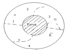
Рисунок 14.1

Для кожного значення U існує певне критичне значення магнітної індукції B_cr, при якому траєкторія електронів тільки торкається поверхні анода. Електрони в цьому випадку практично не досягають аноду, і анодний струм І_а ≈ 0. Коли В = B _cr, радіус траєкторії електрона дорівнює половині радіуса анода (соленоїда) r = R/2.

Індукція магнітного поля в соленоїді визначається за формулою

, (14.7)

де магнітна стала; n – число витків соленоїда, що припадає на одиницю його довжини; сила струму в соленоїді. Коли струм соленоїда наближається до значення, що відповідає індукції B_cr, анодний струм швидко спадає (рис. 14.2). Це значення I_cr можна наближено визначити, продовжуючи спадаючу ділянку до перетину з віссю абсцис.

Після підстановки B_cr в (14.6) отримуємо остаточно

. (14.8)

Рисунок 14.2

Експериментальна частина

1. Експериментальна установа зібрана за схемою на рис. 14.3.

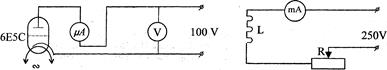
Рисунок 14.3

2. На передній панелі джерела живлення ВУП-2 зліва знаходиться регулятор напруги за допомогою якого можна змінювати значення струму у соленоїді. До включення джерела живлення поставити регулятор на 0, повернувши його проти ходу стрілки годинника до упору.

3. Включити тумблер "СЕТЬ" на випрямлячі ВУП-2.

4. Після нагрівання лампи записати значення напруги U на вольтметрі при відсутності струму в соленоїді.

5. Збільшуючи струм соленоїду від нуля до найбільшого значення через рівні інтервали, зафіксувати відповідні значення анодного струму I_а. Результати занести у таблицю 14.1.