


A purpose of the work is to measure resistance of a conductor by different methods, to calculate the specific resistance, to examine relation Rp= f(1).
Instrumentation and appliances: an experimental plant.
Theoretical part
1. The ordered motion of electric charges is called the electric current. An electric current in metals is the motion of the conductivity electrons. In conducting solutions (electrolytes) ions are the mobile charges. The ions and the electrons carry charges in gases.
Intensity and density are the quantative characteristics of the electrical current. Intensity of current is the charge dq passesthrough a cross section of a conductor in a time dt:
 .
.
If the same amount of electric charges flows through any section of conductor at the equal period of time, the current intensity is constant value I= dq/dt = const. If the current changes by time, it is alternating current dq/dt≠const. The intensity of current is a scalar value and measured in amperes in the SI system. Current intensity is measured in milliamperes ( mA ) and microamperes ( μA ) too.
If current is assigned irregularly along the surface S, then the current density j is defined in every point of the surface. The current density is the ratio
 ,
,
where dS is an area perpendicular to the current direction dI which goes through this area.
The current intensity I through the given surface S can be found with the help of integration:
 .
.
If the current I is assigned regularly through the given surface S then the current density- j=I/S=const. The current density is a vector value and inSI system measured in amperes divided by square meter ( A/m2 ).
The density of a charge j can be assigned by concentration of the charges, itТs value and velocity
 .
.
2. There is relationship between the voltage U applied to the ends of the conductor and the current in it for each conductor if the condition of the conductor is invariable:
 . (8.1)
ItТs the OhmТs law for the part of the electric circuit in integral form. According to the OhmТs law in the differential form j=σE the current density j in the conductor is directly proportionate to the electric intensity E in it, where σ is specific electroconductivity of the conductor. The OhmТs law for the closed circuit is
 ,
,
where ε - electromotive force,
R - external resistance of the conductor,
r - internal resistance of current source.
When the current passes through the conductor, the latter is being heated. The quantity of the produced heat in the conductor is proportionate to its resistance, square value of current intensity and time:
 . (8.2)
If the current intensity changes in time, then:
 . (8.3)
The formulas (8.2) and (8.3) represent the Joule-LenzТ law. The heat quantity Q, which turns from the volume unit into the time unit of the conductor, is called the power of the current. The Joule-LenzТ law in differential form is:
 .
.
3. Simple electric circuits are closed loops. The calculation of the ramified electric circuit is more complex but significantly simplified if we use KirchhoffТs laws.
|
|
|
The first law deals with the junction points and states: the algebraic sum of the currents at any junction point equals to zero (Fig. 8.1). For the junction point A:

or - I 1- I 2+ I 3=0.
The second law deals with electric circuits: for any closed loop the algebraic sum of all incidences of voltage IiRi is equal to the algebraic sum of all the electromotive forces εi in this circuit.
For the 1 circuit
 .
.

Figure 8.1
For the 2 circuit
 .
.
4. The conductorТs resistance is directly proportional to its length and inversely proportional to its cross-section area
 , (8.4)
where ρ - the specific resistance of the conductor,
l - the length of the conductor,
S - cross-section area.
The conductors in the electric field can be connected in series and parallel.
When the conductors connected in series the current has the same value of I (fig. 8.2).
Voltage drop in each resistance
 ;
;  ;
;  .
.

Figure 8.2
Adding right and left parts of these equations we obtain:
 .
.
Hence it follows, that for any n amount of resistances connected in series there is a common resistance:
 . (8.5)
In case of parallel resistance the common current I is branched into  currents.
Let us consider parallel connection for three conductors (fig. 8.3):

Figure 8.3
Voltage drop in each resistance is the same:
 ;
;
 ;
;  ;
;  ;
;  ;
; 
 .
.
In general for n amount of the conductors connected in parallel the total resistance may be expressed by the formula
 .
.
Experimental part
An experimental device to measure the resistance consists of the column with wire and measuring block (fig.8.4).
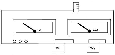
Figure 8.4
On the column there are two motionless brackets and a traveling one which can move along the column and be fixed in any position. The mark which is drawn between the upper and the lower brackets facilitates to define the length of the segment of resisting wire being measured.
The measuring part is placed in the separate block which has milliamperemeter, voltmeter and operating keys. Milliamperemeter is plugged in the resisting wire circle and used to measure the current and voltmeter to measure the voltage in the measured length of resisting wire. The switch W 1 is used to choose the type of work and the switch W 2 to choose the accuracy of current and voltage measurement.
1. Move the traveling bracket for 0,7 - 0,8 of length of the resisting wire, take it from the basis.
2. Press button W 1 Ућ≈–≈∆јФ.
3. Press button W3 Ућ≤—“ќ Ф.
4. When pressing button W2 the scheme works in the Fig. 8.5.

Figure 8.5
5. Write down the measurements which shows millliamperemeter and voltmeter and calculate R using the formula  , Ra = 0,15 Om, Ra = 2500 Om.
6. When pressing button W 2, the scheme in the Fig. 8.6 works.
7. Make measurements of the millliamperemeter and voltmeter readings and calculate R using the formula:
 ,
,  .
.
Figure 8.6
8. Measure with micrometer the diameter of the wire d, the length of the wire from the basis to the traveling contact l, calculate the specific resistance r using the formula
 .
.
9. Using one of the schemes of connection build up the constant value of the current I with the help of regulator. Moving the traveling contact of the resisting wire for a few marks find 8-10 values of the U.
|
|
|
10. Count 8-10 values of R using the formula which correspond to the switching on scheme.
11. Fill in the table with data:
| є | |||||||||
| Ia, A | |||||||||
| I, m | |||||||||
| U v,V | |||||||||
| Rp, Om |
12. Build up the graph Rp =f(I).
13. Count the error for Rp. Make a conclusion about the work done.
Control questions
1. What is an electric current? Write the formula for the direct current.
2. Write the definition and formula for the alternating current.
3. Write the definition and formula for the current density.
4. Write the relationship between the current intensity and its density.
5. Write the OhmТs law in integral form.
6. Write the relationship between the conductor resistance and conductor electroconductivity.
7. Write the OhmТs law for the closed circuit.
8. Formulate and write the Joule LenzТ law.
9. Formulate and write the first and the second KirchhoffТs laws.
10. Write the dependence of the conductor resistance on its cross-section.
11. Deduce the formula for counting two resistors connected in series and parallel.
This instruction is worked out by S. Lushchin, reader of the physics chair.
Reviewer: S. Loskutov, professor of the physics chair.
ЋјЅќ–ј“ќ–Ќј –ќЅќ“ј є 22.2
¬»ћ≤–ё¬јЌЌя ≈Ћ≈ “–»„Ќ»’ ќѕќ–≤¬
ћ≈“ќƒќћ ћ≤—“ ј ”≤“—“ќЌј
ћета роботи: визначити нев≥дом≥ опори методом м≥стка ”≥тстона.
ѕрилади ≥ обладнанн€: реохорд, магазин опор≥в, два нев≥домих опора, нуль-гальванометр, акумул€тор, ключ.
“еоретична частина
≈лектричним струмом називаЇтьс€ будь-€кий впор€дкований (спр€мований) рух електричних зар€д≥в. ” пров≥днику п≥д д≥Їю прикладеного електричного пол€  в≥льн≥ електричн≥ зар€ди перем≥щуютьс€: позитивн≥ по полю, негативн≥ Ц проти пол€, тобто в пров≥днику виникаЇ електричний струм, €кий називаЇтьс€ струмом пров≥дност≥. ƒл€ виникненн€ ≥ ≥снуванн€ електричного струму необх≥дно: 1) на€вн≥сть в≥льних нос≥њв струму Ц зар€джених частинок, здатних перем≥щуватис€ впор€дковано; 2) на€вн≥сть електричного пол€, енерг≥€ €кого, поповнюючись, витрачаЇтьс€ на впор€дкований рух.
”загальнений закон ќма дл€ неоднор≥дноњ д≥л€нки кола представл€Їтьс€ виразом
 , (9.1)
де I Ц струм на д≥л€нц≥ кола 1-2, ε12 Ц ≈–—, що д≥Ї на ц≥й д≥л€нц≥, φ1-φ2 Ц р≥зниц€ потенц≥ал≥в к≥нц≥в д≥л€нки, R Ц оп≥р д≥л€нки кола. якщо на дан≥й д≥л€нц≥ кола джерело струму в≥дсутнЇ (ε12 = 0), то приходимо до закону ќма дл€ однор≥дноњ д≥л€нки кола:
 (9.2)
(9.2)
якщо коло замкнене, тобто точки 1 ≥ 2 сп≥впадають (φ1=φ2), отримуЇмо закон ќма дл€ замкненого кола:
 , (9.3)
де ε Ц ≈–—, що д≥Ї в кол≥, R Ц сумарний оп≥р всього кола. R = r + R1, r Ц внутр≥шн≥й оп≥р джерела струму, R1 Ц оп≥р зовн≥шнього кола.
ƒл€ розрахунку розгалуженого кола, що м≥стить дек≥лька замкнених контур≥в (контури можуть мати сп≥льн≥ д≥л€нки, кожен з них може мати к≥лька джерел струму ≥ т. д.) використовують правила ирхгофа.
Ѕудь-€ка точка розгалуженн€ кола, в €к≥й сходитьс€ не менше трьох пров≥дник≥в ≥з струмом, називаЇтьс€ вузлом. —трум, що входить у вузол, вважаЇтьс€ позитивним, а струм, €кий виходить з вузла, Ц негативним. ѕерше правило ирхгофа: алгебрањчна сума струм≥в, що сход€тьс€ у вузл≥, дор≥внюЇ нулю:
 . (9.4)
ƒруге правило ирхгофа: у будь-€кому замкненому контур≥, вибраному в розгалуженому електричному кол≥, алгебрањчна сума добутк≥в сили струму Ik ≥ опору Rk, що в≥дпов≥дають д≥л€нц≥ контуру м≥ж двома вузлами, дор≥внюЇ алгебрањчн≥й сум≥ ≈–— εk, що д≥ють в цьому контур≥:
|
|
|
 . (9.5)
ƒл€ визначенн€ опор≥в в робот≥ використовують м≥сток ”≥тстона (рис. 9.1), де R x Ц нев≥домий оп≥р, R Ц магазин опор≥в, ADB Ц рео-

хорд.
–исунок 9.1
ћ≥стком Ї галузь —D, що м≥стить гальванометр G. якщо замкнути ключ , струм в≥д джерела ≈ буде йти по розгалуженому колу ≥ м≥стку —D. «м≥нюючи оп≥р магазину, можна дос€гти того, щоб по м≥стку —D струм не йшов. ¬ цьому випадку потенц≥али точок — ≥ D будуть однаков≥. ќднаковими будуть також ≥ р≥зност≥ потенц≥ал≥в м≥ж точками ј ≥ —, ј ≥ D. ≤з закону ќма (9.2) випливаЇ
 , (9.6)
де ≤1 та ≤2 Ц сила струму на д≥л€нках ј— ≥ јD, в≥дпов≥дно.
јналог≥чно, з однаковост≥ р≥зност≥ потенц≥ал≥в м≥ж точками — ≥ ¬, D ≥ ¬ випливаЇ, що
 . (9.7)
ѕод≥ливши (9.6) на (9.7), отримуЇмо
 , (9.8)
де R1 ≥ R2 Ц опори д≥л€нок дроту реохорду зл≥ва ≥ справа в≥д його движка (ковзаючого контакту).
ќп≥р дроту знаходитьс€ за формулами
 ,
,  , (9.9)
де ρ Ц питомий оп≥р матер≥алу дроту, S Ц площина його перетину, l1 ≥ l2 Ц довжини плечей реохорду (в≥дстань в≥д к≥нц≥в реохорду до його движка). “од≥ з формул (9.8), (9.9) знаходимо, що
 . (9.10)
≈кспериментальна частина
1. «≥брати схему (рис. 9.1), використавши в €кост≥ R x один з нев≥домих опор≥в, що Ї в на€вност≥.
2. ƒвижок поставити посередин≥ реохорду на под≥лку 50,0.
3. ѕ≥сл€ перев≥рки схеми викладачем за допомогою магазину опор≥в п≥д≥брати такий оп≥р R, при €кому стр≥лка гальванометра стане на нуль (коли ключ замкнений). ÷е значенн€ R, а також l1 ≥ l2, занести в перший р€док таблиц≥ 9.1.
4. «м≥стити движок реохорду на под≥лку 30,0 ≥ знову, зм≥нюючи оп≥р магазину, знайти значенн€, що в≥дпов≥даЇ нульовому струму. «наченн€ R, l1 ≥ l2 занести в другий р€док таблиц≥.
5. ¬становити движок на под≥лку 70,0, знайти значенн€ R ≥ занести його в трет≥й р€док таблиц≥ разом з l1 ≥ l2.
6. “ак≥ ж сам≥ вим≥ри провести ≥ дл€ другого нев≥домого опору, а пот≥м також дл€ посл≥довно ≥ паралельно зТЇднаних опор≥в Rx1 ≥ Rx2. –езультати вс≥х вим≥р≥в занести в таблицю 9.1.
“аблиц€ 9.1
| ќп≥р | Ќомер вим≥ру i | –езультати вим≥р≥в | Rx(i), ќм | Rx(cp), ќм | ||
| R(≥), ќм | l1(≥), м | l2(≥), м | ||||
| Rx1 | ||||||
| Rx2 | ||||||
| ѕосл≥довне зТЇднанн€ Rx посл | ||||||
| ѕаралельне зТЇднанн€ Rx пар | ||||||
7. «а даними таблиц≥ 9.1, користуючись формулою (9.10), розрахувати Rx(i), а також середнЇ значенн€ Rx(cp) дл€ обох нев≥домих опор≥в та њх посл≥довного ≥ паралельного зТЇднанн€. «анести результати у в≥дпов≥дн≥ стовпчики таблиц≥ 9.1.
8. ористуючись значенн€ми Rx1(cp) ≥ Rx2(cp), розрахувати оп≥р њх посл≥довного та паралельного зТЇднанн€ за формулами
Rпосл = Rx1(cp) + Rx2(cp), Rпар = Rx1(cp) Rx2(cp) /(Rx1(cp) + Rx2(cp)). (9.11)
ѕор≥вн€ти результати цих розрахунк≥в з результатами безпосередн≥х вим≥р≥в Rx посл(cp), Rx пар(cp) (див. таблицю 9.1).
9. ќц≥нити похибку визначенн€ опор≥в методом м≥стка ”≥тстона, наприклад, за результатами вим≥рювань Rx1.
|
|
|
онтрольн≥ запитанн€
1. ўо таке сила струму, потенц≥ал ≥ напруга?
2. ƒати визначенн€ електроруш≥йноњ сили (≈–—).
3. —формулювати закон ќма дл€ однор≥дноњ д≥л€нки кола.
4. —формулювати закон ќма дл€ замкненого кола.
5. ¬ чому пол€гаЇ перше правило ирхгофа?
6. яке друге правило ирхгофа?
7. Ќамалювати схему м≥стка ”≥тстона ≥ по€снити, €к за його допомогою можна визначити нев≥домий оп≥р.
8. ѕо€снити, чому при в≥дсутност≥ струму кр≥зь гальванометр пад≥нн€ напруги на д≥л€нках ј— ≥ јD однакове.
9. ƒати по€сненн€, чому, коли гальванометр показуЇ нуль, струм кр≥зь опори R ≥ Rx однаковий?
Ћ≥тература
1. “рофимова “.ј. урс физики. ћ.: ¬ысша€ школа, 1999.
2. —авельев ».¬. урс общей физики. -ћ.: Ќаука, 1989. ІІ 35, 36.
3. ƒетлаф ј.ј., яворский Ѕ.ћ. урс физики. -ћ: ¬ысша€ школа, 1989.
≤нструкц≥€ складена проф. кафедри ф≥зики Ћоскутовим —.¬.
–ецензент: доц. кафедри ф≥зики ™ршов ј.¬.
ЋјЅќ–ј“ќ–Ќј –ќЅќ“ј є 23
ƒќ—Ћ≤ƒ∆≈ЌЌя ≈Ћ≈ “–ќ—“ј“»„Ќќ√ќ ѕќЋя
Ќј ћќƒ≈Ћ≤
ћета роботи: побудувати екв≥потенц≥альн≥ та силов≥ л≥н≥њ електростатичного пол€ та розрахувати його напружен≥сть.
ѕрилади ≥ обладнанн€: джерело живленн€, потенц≥ометр, панель з електродами та електропров≥дним папером, зонд, осцилограф.
“еоретична частина
≈лектростатичне поле створюЇтьс€ нерухомими електричними зар€дами ≥ визначаЇтьс€ в кожн≥й точц≥ простору силою, що д≥Ї на пробний зар€д.
√оловна характеристика електростатичного пол€ Ц його напружен≥сть:
 , (10.1)
де  Ц сила, €ка д≥Ї на точковий зар€д q, внесений в дану точку простору.
≈нергетичною характеристикою електростатичного пол€ Ї електростатичний потенц≥ал U. ¬≥н визначаЇтьс€ роботою, €ку виконуЇ електрична сила при перем≥щенн≥ одиничного позитивного зар€ду з даноњ точки в неск≥нченн≥сть.
оли зар€д перем≥щуЇтьс€ з дов≥льноњ точки 1 в дов≥льну точку 2, виконана при цьому робота не залежить в≥д траЇктор≥њ ≥ визначаЇтьс€ т≥льки р≥зницею потенц≥ал≥в:
 . (10.2)
ѕотенц≥ал Ї функц≥Їю координат  . якщо розпод≥л потенц≥алу в≥домий, можна знайти напружен≥сть:
 , (10.3)
де оператор grad в прав≥й частин≥ називаЇтьс€ град≥Їнтом. ¬≥н д≥Ї на скал€рну функц≥ю координат  за правилом:
 , (10.4)
 Ї одиничн≥ вектори вздовж осей x, y ≥ z, в≥дпов≥дно.
≈лектростатичне поле можна зобразити за допомогою екв≥потенц≥альних поверхонь (екв≥потенц≥альних л≥н≥й в двохвим≥рному випадку). ≈кв≥потенц≥альна поверхн€ (л≥н≥€) Ц це геометричне м≥сце точок однакового потенц≥алу.
ƒл€ зображенн€ електростатичного пол€ можна також використати силов≥ л≥н≥њ (л≥н≥њ напруженост≥). —иловою л≥н≥Їю називаЇтьс€ л≥н≥€, дотична до €коњ в кожн≥й точц≥ сп≥впадаЇ з вектором напруженост≥. ѕри побудов≥ силових л≥н≥й можна використати так≥ њх властивост≥:
а) силов≥ л≥н≥њ починаютьс€ на позитивних зар€дах ≥ зак≥нчуютьс€ на негативних (або розс≥юютьс€ в неск≥нченност≥);
б) силов≥ л≥н≥њ при перетин≥ екв≥потенц≥альних поверхонь (л≥н≥й) спр€мован≥ перпендикул€рно до них;
в) оск≥льки зар€джен≥ металев≥ поверхн≥ Ї екв≥потенц≥альними, силов≥ л≥н≥њ виход€ть (або вход€ть) перпендикул€рно до електрод≥в;
г) силов≥ л≥н≥њ розташован≥ густ≥ше в тих м≥сц€х, де б≥льше напружен≥сть;
д) силов≥ л≥н≥њ спр€мован≥ в б≥к зменшенн€ потенц≥алу.
≤снуЇ аналог≥€ м≥ж розпод≥лом потенц≥алу електростатичного пол€ в однор≥дному д≥електричному середовищ≥ та розпод≥лом потенц≥алу в однор≥дному пров≥днику з електричним струмом. ÷е можна по€снити тим, що обидва випадки описуютьс€ тим же самим р≥вн€нн€м, €ке не включаЇ жодного параметру середовища
 . (10.5)
÷е р≥вн€нн€ може бути застосоване до д≥електрика так же само, €к до пров≥дника. ћожна вивчати електричне поле в д≥електрику шл€хом вим≥рюванн€ розпод≥лу потенц≥алу в пров≥днику, хоч цей розпод≥л потенц≥алу маЇ зовс≥м ≥нше походженн€.
≈кспериментальна частина
–озпод≥л потенц≥алу в тонкому пров≥дному шар≥ використовуЇтьс€ в ц≥й робот≥ в €кост≥ двохвим≥рноњ модел≥ електростатичного пол€. ƒл€ вим≥рюванн€ потенц≥алу використовуЇтьс€ м≥сткова схема (рис. 10.1). ƒва метал≥чних електроди ј ≥ ¬ притиснут≥ до аркуша паперу з пров≥дним шаром. Ќапруга U o = 6,3 ¬ в≥д джерела живленн€ подаЇтьс€ на електроди ≥ на нижн≥ клеми потенц≥ометра. ƒо рухомого контакту S через клеми вертикального в≥дхиленн€ осцилографа (вх≥д Y) приЇднуЇтьс€ зонд P.

¬ робот≥ осцилограф використовуЇтьс€ в €кост≥ ≥ндикатору на€вност≥ р≥зниц≥ потенц≥ал≥в. оли зонд доторкаЇтьс€ поверхн≥ пров≥дного паперу, на осцилограф≥ спостер≥гаЇтьс€ сигнал (у вигл€д≥ вертикального в≥др≥зку, висота €кого пропорц≥йна р≥зниц≥ потенц≥ал≥в м≥ж точкою дотику зонда та контактом S). оли потенц≥ал в точц≥ дотику дор≥внюватиме потенц≥алу на рухомому контакт≥, на екран≥ будемо спостер≥гати точку.
|
|
|
–исунок 10.1
Ќа початку роботи п≥д електроди та пров≥дний пап≥р вм≥щують два-три аркуш≥ паперу, на кожному з €ких ол≥вцем обведено по контуру електроди, притиснут≥ в тому положенн≥, в €кому вони будуть знаходитись п≥д час роботи.
Ѕудемо вважати, що потенц≥ал точки ј дор≥внюЇ нулю U ј = 0. “од≥ U ¬ = 6,3 ¬ (приймаЇтьс€ до уваги т≥льки ампл≥тудне значенн€ потенц≥алу). ƒл€ того, щоб отримати екв≥потенц≥альну л≥н≥ю дл€ певного значенн€ потенц≥алу 0 < Ui < 6,3 ¬, треба спочатку перевести рухомий контакт S у в≥дпов≥дне положенн€ d i:
 , (10.6)
де d 0 Ц довжина робочоњ частини потенц≥ометра (намотки). ƒал≥ необх≥дно перем≥щувати зонд по поверхн≥ пров≥дного паперу у напр€мку зменшенн€ сигналу ≥ зупинити його, коли сигнал буде дор≥внювати нулю. ѕотенц≥ал в точц≥ зупинки дор≥внюЇ Ui. ўоб заф≥ксувати положенн€ ц≥Їњ точки, треба проколоти пап≥р гострим к≥нцем зонда.
ѕор€д з ц≥Їю точкою треба знайти ще одну точку з потенц≥алом Ui ≥ заф≥ксувати њњ, щоб, посл≥довно перем≥щуючись в≥д одн≥Їњ точки до ≥ншоњ, отримати низку прокол≥в на аркушах паперу, за €кими можна пот≥м побудувати екв≥потенц≥альну л≥н≥ю, коли аркуш≥ буде вийн€то.
1. ќтримати екв≥потенц≥альн≥ л≥н≥њ, задаючи значенн€ потенц≥алу в≥д 0 до 6,3 ¬ з кроком 0,9 ¬. ѕрийн€ти до уваги, що контури електрод≥в Ї екв≥потенц≥альними л≥н≥€ми, що в≥дпов≥дають значенн€м потенц≥алу 0 ≥ 6,3 ¬.
2. ѕобудувати систему силових л≥н≥й (к≥льк≥стю не менше, н≥ж 7).
3. ¬изначити величину ≥ напр€мок напруженост≥ пол€ в к≥лькох точках, €к≥ задаЇ викладач. ¬еличину напруженост≥ можна знайти за наближеною формулою
 , (10.7)
де Un ≥ Un+1 Ї значенн€ потенц≥алу двох екв≥потенц≥альних л≥н≥й, найближчих до точки, в €к≥й визначаЇтьс€ напружен≥сть; D Ц довжина найкоротшого в≥др≥зку, що зТЇднуЇ ц≥ л≥н≥њ ≥ проходить кр≥зь дану точку.
4. ќц≥нити помилку, з €кою визначено положенн€ екв≥потенц≥альних л≥н≥й, за формулою
 , (10.8)
де k (¬/под≥лку) Ц положенн€ д≥льника на вход≥ Y осцилографа.
онтрольн≥ запитанн€ та вправи
1. ƒайте визначенн€ напруженост≥ та потенц≥алу електростатичного пол€. ¬ €ких одиниц€х вим≥рюютьс€ ц≥ величини?
2. як зв'€зан≥ м≥ж собою напружен≥сть пол€ ≥ потенц≥ал?
3. „ому поверхн€ пров≥дника Ї екв≥потенц≥альною?
4. як≥ л≥н≥њ називаютьс€ силовими? як≥ њх властивост≥?
5. ƒовед≥ть, що силов≥ л≥н≥њ перпендикул€рн≥ до екв≥потенц≥альних поверхонь.
6. —формулюйте теорему ќстроградського-√ауса.
7. ѕокаж≥ть, що потенц≥ал точкового зар€ду  задовольн€Ї р≥вн€нню (10.5).
8. ќтримайте наближене сп≥вв≥дношенн€ (10.7) з точноњ формули (10.3).
9. ѕ≥дтвердить, що помилка в положенн≥ екв≥потенц≥альних л≥н≥й може бути оц≥нена за формулою (10.8).
Ћ≥тература
1. “рофимова “.ј. урс физики. -ћ.: ¬ысша€ школа, 1999, ІІ 77-86.
2. —авельев ».¬. урс общей физики. -ћ.: ¬ысша€ школа, 1998, т. II, ІІ 1.1-1.14.
3. «исман √.ј., “одес ќ.ћ. урс общей физики. -ћ.: Ќаука, 1972, т. II, ІІ1.4-1.8.
4. ƒетлаф ј.ј., яворский Ѕ.ћ. урс физики. -ћ: ¬ысша€ школа, 1989. ІІ 13.1-13.5
.
≤нструкц≥€ складена ст. викл. каф. ф≥зики ƒенисовою ќ.≤.,
в≥дредагована доц. каф. ф≥зики урбацьким ¬.ѕ.
–ецензент: доц. кафедри ф≥зики ™ршов ј.¬.
LABORATORY WORK є 23

