


ќ“„≈“
| ћесто прохождени€ практики: | ‘√Ѕќ” ¬ѕќ Ђ ам√” им. ¬итуса Ѕерингаї | |||
| афедра математики и физики | ||||
| ¬ыполнил студент группы ѕћм - 14 | ƒ.¬. ћакаров | |||
| (ѕодпись студента) | ||||
| –уководитель практики профессор кафедры информатики, доктор технических наук. | ё.¬. ћарапулец | |||
| (ѕодпись руководител€) | ||||
| –уководитель практики от предпри€ти€ андидат физико-математических наук, доцент кафедры математики и физики. | –.». ѕаровик | |||
| (ѕодпись руководител€) | ||||
| ќтчет защищен Ђ____ї___ 2016 г. с оценкой ____________________ | ||||
| (ѕодпись руководител€) | ||||
г. ѕетропавловск- амчатский, 2016 г.
»ндивидуальный план
преддипломной практики
студента ћакаров ƒ.¬.
гр. ѕћм - 14
| Ётап | ¬ид работ | —роки | –езультат / ‘орма представлени€ результата |
| ќрганизационный | ‘ормулировка конкретного исследовательского задани€. —оставление индивидуального плана работ. | 28 марта Ц 4 апрел€ | онкретизаци€ направлений исследовани€ и составление индивидуального плана работы. |
| ќзнакомительный | —оставление обзора Ќ»–. јнализ исследований в предметной области. | 4 апрел€ Ц 11 апрел€ | ќбзор научной литературы в исследуемой области. Ќаписание научной статьи. |
| јктивный | ѕроведение исследований в соответствии с планом. ”частие в семинаре в Ќ»» прикладной математики и автоматизации г. Ќальчик | 11 апрел€ Ц 16 ма€ | ѕредставление научной статьи, соответствующей плану исследований и теме диссертации. |
| «авершающий | «авершение всех видов работы. —оставление и оформление отчета по практике. ѕодготовка отчетных документов (характеристик и пр.) | 16 ма€ Ц 29 ма€ | ќтчет по практике, ћагистерска€ диссертаци€, –укописи статей. |
—ќƒ≈–∆јЌ»≈
| »Ќƒ»¬»ƒ”јЋ№Ќџ… ѕЋјЌ ѕ–≈ƒƒ»ѕЋќћЌќ… ѕ–ј “» »Е.. | |
| ¬¬≈ƒ≈Ќ»≈ЕЕЕЕЕЕЕЕЕЕЕЕЕЕЕЕЕЕЕЕЕЕЕЕЕ. | |
| ќ—Ќќ¬Ќјя „ј—“№ЕЕЕЕЕЕЕЕЕЕЕЕЕЕЕЕЕЕЕЕЕ.. | |
| 1. “еоретико-методологические основы развити€ теории длинных волн Ќ.ƒ. ондратьеваЕЕЕЕЕЕЕЕЕЕЕЕЕЕЕЕЕЕЕЕЕ. | |
| 1.2 ћетодологические подходы к исследованию длинных волнЕЕ. | |
| 1.3 ’арактеристика исследований, проводимых в рамках индивидуального плана практикиЕЕЕЕЕЕЕЕЕЕЕЕЕ.. | |
| 2. »—’ќƒЌџ≈ ƒјЌЌџ≈ »——Ћ≈ƒќ¬јЌ»яЕЕЕЕЕЕЕЕЕЕ | |
| 2.1 ќбзор проблемной областиЕЕЕЕЕЕЕЕЕЕЕЕЕЕЕЕ | |
| 3. ѕЋјЌ —јћќ—“ќя“≈Ћ№Ќџ’ »——Ћ≈ƒќ¬јЌ»…ЕЕЕЕЕЕЕ. | |
| 4. –≈«”Ћ№“ј“џ —јћќ—“ќя“≈Ћ№Ќџ’ »——Ћ≈ƒќ¬јЌ»…ЕЕЕ... | |
| 4.1 ќбобщенна€ модель ƒубовского, с учетом эффекта пам€ти в экономической системеЕЕЕЕЕЕЕЕЕЕЕЕЕЕЕЕЕЕ. | |
| 4.2 јлгоритм реализаци€ моделировани€ в компьютерной среде MatlabЕЕЕЕЕЕЕЕЕЕЕЕЕЕЕЕЕЕЕЕЕЕЕЕЕ.. | |
| «ј Ћё„≈Ќ»≈ЕЕЕЕЕЕЕЕЕЕЕЕЕЕЕЕЕЕЕЕЕЕЕ.. | |
| —ѕ»—ќ Ћ»“≈–ј“”–џЕЕЕЕЕЕЕЕЕЕЕЕЕЕЕЕЕЕЕ.. | |
| ѕ–»Ћќ∆≈Ќ»≈ ј Ц —писок научных публикацийЕЕЕЕЕЕЕЕЕ |
|
|
|
¬¬≈ƒ≈Ќ»≈
ѕреддипломна€ практика была пройдена мною на базе кафедры физики и математики физико-математического факультета ам√у им. ¬итуса Ѕеринга.
÷ель преддипломной практики Ц проведение самосто€тельного исследовани€, подготовка квалификационной работы Ц магистерской диссертации, заключающей в своем составе результаты индивидуального исследовани€.
¬ соответствии с целью были поставлены и решены во врем€ прохождени€ преддипломной практики, следующие задачи:
- планирование научно-исследовательской работы;
- сбор материалов дл€ магистерской диссертации, обзор исследований в проблемной области;
- обоснование актуальности, новизны и практической значимости магистерской диссертации;
- проведение исследовательской работы согласно плану;
- апробаци€ результатов исследовани€ на региональных и всероссийских научных меропри€ти€х;
- подготовка научных статей;
- участие в работе научных коллективов;
- подготовка магистерской диссертации.
–езультативность преддипломной практики проведенной на кафедре физики и математики физико-математического факультета ам√у им. ¬итуса Ѕеринга в разрезе решени€ поставленных задач, в отражена в отчете.
ќ—Ќќ¬Ќјя „ј—“№
1. “еоретико-методологические основы развити€ теории длинных волн Ќ.ƒ. ондратьева.
ѕроцессы формировани€ современной российской экономики во многом идентичны процессам, которые имели место в —Ўј, ¬еликобритании, японии, √ермании в прошлом. ¬не зависимости от временных отставаний развити€ отдельных отраслей и технологий, повышенной чувствительности российской экономики к кризисам, общее развитие все же протекает по закономерност€м, вы€вленным зарубежными и российскими учеными еще во второй половине XIX века.
ѕервые теоретические разработки, имеющие своей основой попытку структурного обобщени€ и систематизации основных принципов развити€ экономических систем и свойственных последним флуктуаций, базируютс€ на научных трудах английского ученого X. ларка [2].
“еоретические постулаты ¬. ƒжевонса сопровождаемые попыткой математического обосновани€, основанного на статистическом анализе множества экономических показателей, не получили широкого признани€ современников ученого, а напротив, вызвали ожесточенный научный спор не затихающий и в насто€щее врем€ о самом существовании каких либо длительных колебаний в экономике и правомерности периодизации последних.
Ѕольшее внимание научной общественности середины XIX века к вопросу о существовании длительных колебаний в экономике и проблематике периодизации последних вызвала разработанна€ . ћарксом в 1860 годах Ђ“еори€ циклических кризисовї. ƒанный труд существенно отличалс€ от фрагментарных теоретических предположений экономистов английской школы, и в первую очередь тем, что не только призывал объективным факт существовани€ феномена длительных колебаний в экономике, но и св€зывал наличие последних с циклами технического прогресса и ростом прибыли капиталистов. Ђ“еори€ циклических кризисовї . ћаркса привнесла импульс к развитию научной мысли учеными-марксистами понимани€ феномена длинных волн на начальном этапе развити€ общей концепции.
«начительно больший вклад в развитие постулатов теории длинных волн привнес русский исследователь-марксист ј.». √ельфанд, впервые сформулировав в 1901 году гипотезу, что длительные периоды экономической экспансии, спада и засто€ имманентны капиталистическому способу производства.
|
|
|
ќсновыва€сь на постулатах теории . ћаркса и собственных научных изыскани€х ј.». √ельфанд вы€вил и обозначил основные причины, предопределившие бурный экономический рост начала XX века, в частности развитие электроэнергетики, увеличение добычи редкоземельных металлов, в основном золота и серебра, по€вление новых рынков [9].
Ќаучные взгл€ды ј.». √ельфанда впоследствии нашли свое продолжение в трудах русского ученого Ќ.ƒ. ондратьева имеющих своей основой попытку структурного обобщени€ и систематизации основных принципов математического моделировани€ поведени€ экономических систем в разрезе феномена Ђдлинных волнї.
Ќаучные исследовани€ и выводы Ќ.ƒ. ондратьева основывались на эмпирическом анализе большого числа экономических показателей различных стран на довольно длительных промежутках времени, охватывавших 100-150 лет [7].
1.2 ћетодологические подходы к исследованию длинных волн.
¬ насто€щее врем€ научный вклад Ќ. ƒ. ондратьева оцениваетс€ двойственно и соответственно интерпретируетс€ па разному. –азличи€ наход€т свое про€вление в подходах ученых зан€тых проблематикой прогнозировани€ длинноволновой динамики в долгосрочном экономическом развитии.
ќдна группа исследователей прибегает к использованию сложных математических моделей (на основе статистических показателей) анализа временных р€дов, друга€ напротив выстраивает мультифакторную модель, пыта€сь охватить весь спектр экономических показателей, а треть€ вовсе не раздел€ет положени€ теории Ќ.ƒ. ондратьева и приводит массу доводов опровергающих научный вклад ученого.
ќднако при всем многообразии подходов и мнений к возможности прогнозировани€ длинноволновой динамики все исследователи едины во мнении, что тенденции развити€ любой экономической системы нос€т циклический характер, т.е. периодический и, следовательно, в нем можно вы€вить некоторые закономерности.
¬ вопросе вы€влени€ вышеозначенных закономерностей исследователи, исход€т из различных предпосылок (механизмов возникновени€ длинных волн) и как следствие используют различные методологические подходы к исследованию длинных волн.
ћарксистское направление исследований длинных волн. ѕервым методологическим подходом априори €вл€етс€ марксистское направление исследований, возникшее в 60-тых годах XIX века. ќсновой дл€ его по€влени€ €вилось эволюционна€ трансформаци€ статичного промышленного капитализма, предопредел€вша€ переход к ускоренному развитию индустриального общества.
этому подходу относ€тс€ исследовани€ циклических процессов на основе экономических моделей, построение которых основывалось на строго определенной группе экономических факторов описываемых с помощью основных характеристик.
ћарксистское направление как вытекает из названи€ св€занно с научными трудами . ћаркса заложившего фундамент дл€ исследовани€ длинноволновых колебаний. . ћаркс впервые рассмотрел циклические колебани€ во взаимодействии с накоплением капитала и изложил концепцию перепроизводства, в разрезе которой выдвинул положение, что именно перепроизводством объ€сн€етс€ возникновение кризисов в капиталистической экономике [11].
ѕоложени€, выдвинутые . ћарксом несколько позднее, послужили основой дл€ вы€влени€ им взаимозависимости роста органического строени€ капитала и падени€ нормы прибыли.
ћарксистское направление исследовани€ длинных волн в экономике основывалось на четырех подходах.
- собственно подход . ћаркса (взаимозависимость роста органического строени€ капитала и падени€ нормы прибыли);
- инвестиционный подход (спрос на капитал);
- неравновесный подход (развитие и направление движение научно-технического прогресса);
- экзогенный подход (совокупность внешних факторов).
ќсновыва€сь на догматических положени€х концепции перепроизводства изложенной . ћарксом объ€сн€ющей генезис кризисов в капиталистической экономике, отдельные представители данного направлени€ ћ.». “уган-Ѕарановский, Ќ.ƒ. ондратьев рассматривали длинноволновые колебани€, придерживались модели инвестиционного цикла и осуществл€ли выбор показателей, рассматрива€ инвестиции в качестве ведущего фактора [6].
|
|
|
»нвестиционный подход просматриваетс€ в научных трудах ћ.». “уган-Ѕарановского в частности в его монографии Ђѕериодические промышленные кризисыї последн€€, представл€ет собой теорию промышленных циклов, содержащую аргументы и выводы в пользу существовани€ цикличности в развитии промышленного производства [].
¬ интерпретации Ќ.ƒ. ондратьева инвестиционна€ модель длинного цикла, по сути, дополн€ла модель . ћаркса.
ќднако Ќ.ƒ. ондратьев в рамках инвестиционной модели длинного цикла существенно развил теорию . ћаркса, предположив, и не безосновательно существование внутреннего эндогенного механизма формировани€ экономической динамики, т.е. больших циклов конъюнктуры.
¬ продолжение инвестиционной модели длинного цикла Ќ.ƒ. ондратьева, в 20-е XX-века годы ƒ.». ќпарин и √. ассель выдвинули концепцию длинных циклов, основанную на изменении количества денег в обращении, позднее данна€ концепци€ получила развити€ в научных трудах …. ƒельбеке и ѕ. орпмена в разрезе позиции ученых, согласно которой в насто€щее врем€ считаетс€, что будущее в исследовании длинных волн принадлежит интегрированию различных моноказуальных (одно-причинных) моделей [8].
…ос ƒельбеке в своих трудах высказал предположение, что многие моноказуальные модели в принципе совместимы. » в качестве обосновани€ своей научной позиции приводит пример научных изысканий французского исследовател€ ј. ѕиатье, который полагал, что при изучении длительных колебаний необходимо опиратьс€ на процессы, порождающие среднесрочные колебани€, принимать во внимание инновационные аспекты, социальные и политические проблемы, предопредел€ющие кардинальное изменение окружающей среды.
¬ развитие инвестиционной модели длинного цикла –оберт —олоу предложил использование модели Ђкривой ростаї дл€ вы€влени€ и прогнозировани€ циклических колебаний. ћодель Ђкривой ростаї –. —олоу перва€ мультифакторна€ модель, включающа€ множество различных аспектов Ц сопоставление хоз€йственного развити€ различных стран, оценка уровн€ и вклада Ќ“ѕ в экономический прогресс и т.д.
»нтерес к модели –. —олоу про€вл€лс€ в 1970 годы XX-века и был вызван проблематикой неравномерности экономического развити€.
“ем не менее, –. —олоу была разработана и предложенна€ математическа€ модель, имеюща€ в общем случае следующий вид (1):
Q' = A' + wk K' + w j L' (1)
где Q' Ц темп прироста объема выпуска;
ј' Ц темп прироста Ќ“ѕ;
K' Ц темп прироста капитала;
L' Ц темп прироста затрат труда;
w k Ц дол€ капитала в совокупном доходе;
w j Ц дол€ труда в совокупном доходе [22].
ќднако модель –. —олоу не была лишена некоторых противоречий, в частности дискуссионными €вл€ютс€ вопросы цикличности процессов роста, замедлени€ и спада в экономике и наличие следующей проблемы: если имеют место долговременные колебани€ объема выпуска Q', то в какой мере они св€заны с колебани€ми параметров рассматриваемой модели Ц затрат труда и капитала, вклада научно-технического прогресса и изменений долей факторов в совокупном доходе?
Ќесовершенство модели –. —олоу удалось и при том достаточно успешно нивелировать ”олтеру ”итменену –остоу.
ћодель ”.”. –остоу сопоставима в отельных положени€х с неоклассическими модел€м делового цикла, предложенна€ модель основывалась на колебани€х кривой роста продукции и делении продукции между основным и промышленным секторами (формальна€ модель ”.”.–остоу Ц ћ. еннеди) [21].
”.”. –остоу в своей модели предложил выделить основные сектора по критерию значимости их вклада и возможности их вли€ни€ на экономику. »сследователь выделил основные сектора экономики: текстильную промышленность, железные дороги, производство электричества и автомобилей, отрасли подверженные циклическим колебани€м роста и выдвинул предположение, что длинноволновые колебани€ св€занны с периодической замещением (интенсификаци€ Ќ“ѕ) одного ведущего сектора другим.
|
|
|
—ущественный вклад в развитие инвестиционной модели длинного цикла так же внес профессор ћассачусетского технологического университета ƒжей ‘оррестер в 1970-е годы XX века. ќсновными постулатами модели ƒж. ‘оррестера выступила адаптаци€ модели делового цикла ƒж. ћ. ейнса предопредел€вша€ доминирующее значение спросу на капитал.
ƒж. ‘оррестер выдвинул гипотезу, что динамика спроса на капитал не только подвержена циклическим колебани€м вызванным необходимостью смены и расширени€ основных капитальных благ, но и оказывает вли€ни€ на цикличность экономического развити€.
¬ поддержку модели ƒж. ‘оррестера выступил американский ученый Ѕрайан Ѕерри убежденный сторонник ценовой концепции длинных волн.
»нновационное направление исследований длинноволной динамики исследовани€, получившие свое развитие в 20-е годы XX века.
ѕредставител€ми инновационного подхода в разное врем€ были ….ј. Ўумпетер, √. ћенш, ј. л€йккнехт, –. Ѕатр, ¬. ¬айдлих, —. ¬ибе, ƒж. √аттеи, ƒж. √олд-стайн, ѕ. орпинен, ». ћиллендорфер, ћ. ќльсен, Ё. —крепанти, Ѕ. —ильвер ё.¬. яковец и многие другие.
»нновационна€ концепци€ длинного цикла имеет своим основанием попытку четкого определени€ состава и структуры экономических показателей позвол€ющую с большей точностью охарактеризовать научно-технический прогресс.
»нновационное направление исследовани€ длинных волн базируетс€ на трех основных подходах к постановке решени€ проблемы:
- подход синтеза (….ј. Ўумпетер);
- подход Ђмодели метаморфозї (√. ћенш);
- подход Ђлидирующего фактораї/Ђлидирующего сектораї (ƒж. √аттеи, ƒж. √олд-стайн, ѕ. орпинен и др.).
ƒоминирующее значение в инновационном направлении, безусловно, отведено научным взгл€дам ….ј. Ўумпетера которые во многом повли€ли на развитие данного направлени€, догматические положени€ научных трудов Ќ.ƒ. ондратьева легли в основу формулировки ….ј. Ўумпетером основных положений Ђ“еории инновацийї и Ђ“еории предпринимательстваї, раскрывающих сущность инноваций и новую роль предпринимател€ в инновационном процессе, а так же введение в научный оборот пон€ти€ Ђинновацииї и ее определени€ как Ђновой научно-производственной комбинации производственных факторовї [19].
Ќаучный вклад ….ј. Ўумпетера в понимание природы циклических колебаний обширен и многогранен. ќсновыва€сь на собственном видении модели циклов ….ј. Ўумпетер разработал и представил четырехфазовую схему, заключающую следующие логически взаимозависимые этапы: подъем → спад (рецесси€) → депресси€ → оживление.
¬ своей модели ….ј. Ўумпетер основываетс€ на синтезе и взаимопроникновении трех циклических волн: 40 мес€цев (цикл итчина (английский экономист ƒжозеф итчин)), 7 Ц 11 лет (цикл ∆югл€ра (французский экономист лемент ∆югл€р)), 40 Ц 50 лет (цикл Ќ.ƒ. ондратьева) основой которой €вл€етс€ неравномерное, св€занное с развитием научно-технического прогресса внедрение инноваций, которые выражаютс€ во введении только новых товаров и форм производства, а также обмена.
¬ развитие идей ….ј. Ўумпетера в 1979 году √. ћенш предлагает нелинейную теоретическую Ђмодель метаморфозї, усовершенствованную версию теории инновационного цикла, сочетающую р€д внутренних факторов дл€ объ€снени€ причин накоплени€ инноваций между фазами спада и подъема и классифицировал нововведени€ (инновации) базисные и улучшающие.
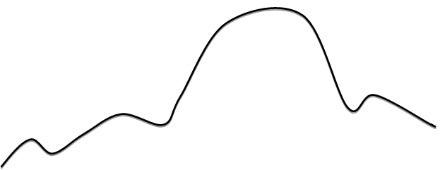
ќсновой модели предложенной √. ћеншом стала гипотеза, что каждый длинный цикл имеет форму S-образной, или логистической, кривой, описывающей траекторию жизненного цикла соответствующего технического способа производства.
“очку сли€ни€ последовательных жизненных циклов √. ћенш определил термином Ђтехнологический патї т.е. периодом структурной трансформации, учитывающим дискретный характер перехода одного длинного цикла в другой, рис.1.


 “очки перелома

“ехнологический пат
–ис.1. ѕоследовательное сли€ние жизненных циклов √. ћенша
ћодель √. ћенша в отношении объ€снени€ причин и механизма длинноволновых колебаний основываетс€ на тезисе что структурное взаимодействие и сочетание базисных и улучшающих инноваций (технических нововведений), априори предполагает наличие некоторой неравномерности (основа жизненный цикл инноваций) оказывающей вли€ни€ на волновые колебани€.
|
|
|
ƒискуссионным пунктом в модели √. ћенша раскрывающим, по мнению исследовател€, механизм длинноволновых колебаний выступает разработанна€ автором схема внедрени€ инноваций, согласно которой доминирующа€ часть инфраструктурных (базисных) нововведений сосредотачиваетс€, как правило, в фазе депрессии длинной волны [18].
¬ продолжение теоретических изысканий √. ћенша ј. лайнкнехт предложил периодизацию возникновени€ кластеров базисных инноваций на основе создани€ многофакторной модели экономического развити€ включающей в своем составе р€д экономико-политических факторов в частности: трудовые ресурсов (их качество и количество), государственна€ экономическа€ политика, внешнеэкономические услови€, уровень развити€ и инвестиционна€ ориентаци€ финансовых институтов, уровень развити€ национальной экономики и т.д.
ј. лайнкнехт в сотрудничестве с исследователем Ѕьешарам обнаружили некоторые недостатки в своей теории и в 1983 г. пытались нивелировать последние посредством применени€ метода приближенного к подходу учинского и ¬ан дер ÷вана, согласно которому длинные волны рассматриваютс€ в виде последовательности относительно долгих периодов подъема экономики (Ђподъемыї, или Ђј периодыї) и ее упадка (Ђспадыї, или Ђ¬ периодыї).
¬ том случае, когда гипотеза длинных волн релевантна, возможно продемонстрировать, что средние темпы роста дл€ так называемых ј периодов большого цикла значительно выше, чем средние темпы роста предыдущих и последующих ¬ периодов и наоборот. —редние темпы роста вычисл€лись дл€ разных временных циклов промышленного производства и валового продукта дл€ разных стран, а также дл€ двух циклов мирового промышленного производства.
ј. лайнкнехт указывает на то, что модель, разработанна€ им ранее в соавторстве с Ѕьешаром, Ђне дает доказательств существовани€ -волн как действительных цикловї и не объ€сн€ет эндогенность перехода от ј к ¬ периодам и обратно. »менно поэтому ј. лайнкнехт вводит в анализ темпов промышленного роста инновационную теорию √. ћенша и в последующих работах основываетс€ на патентной статистике.
—татистическа€ основа дл€ данных циклов, как подчеркивали в своих работах авторы, не была проверена. Ѕьешар и ј. лайнкнехт выполнили оценку средних темпов роста дл€ ј и ¬ периодов большого цикла путем расчета логарифмических трендов в первоначальных циклах.
ѕри расчете трендов учитывались следующее ограничение Ц в переходные годы (годы пика и максимального спада в пределах большого цикла) примерные значени€ трендов дл€ предшествующих и последующих периодов должны совпадать. Ёто согласуетс€ с предложением, что во врем€ перехода от ј к ¬ периодам и наоборот не может быть неравномерных скачков дл€ абсолютного уровн€ переменных.
¬ математических терминах модель лайнкнехта и Ѕьешара может быть изложена следующим образом (2-4):
T0 Ц первый год периода;
Tm Ц последний год периода;
T1, T2,...,Tm-1 Ц промежуточные годы.
“огда линейный тренд за i-й период может быть выражен формулой:
Ln yt = ai + bit дл€ Ti-1, Ti-1 + 1,..., Ti. (2)
ќграничени€ дл€ тренда описываютс€ как:
ai + biTi = ai + 1 + bi+1 Ti, дл€ I = 1,2,..., m-1.
ѕосле определени€ начальных условий Y0 = a1+ biT0 и Yi = ai + biTi дл€ I = 1,..., m модель приобретает вид:
Ln yt = yi-1 + (t Ц Ti-1)  дл€ t = Ti-1, Ti-1 + 1,..., Ti, (3)
или
Ln yt =  yi-1 +
  yi. (4)
¬ последнем выражении Ln y представл€ет собой взвешенную сумму значений в начальном и конечном году рассматриваемого периода. ”казанные выше ограничени€ требуют, чтобы все yi рассматривались одновременно. ¬ конечном итоге были рассмотрены логарифмические тренды дл€ разных ј и ¬ периодов, при которых налагаемые ограничени€ гарантируют непрерывный рисунок Ђзигзагаї. ”казанные выше yi представл€ют собой расчетные значени€ в переходные годы [10].
ќтечественные представители инновационного подхода Ћ.ј. лименко, —.ё. √лазьев, ё.¬. яковц в рамках расширени€ и дополнени€ инновационной концепции длинного цикла раздел€ют инновации на классификационные группы.
¬ частности ё.¬. яковец выделил четыре основных группы инноваций:
- базисные инновации, формирующие новые направлени€ развити€ техники и технологии;
- инновации, стимулирующие переход к новому поколению техники в рамках одного направлени€;
- нововведени€, на основе которых создаютс€ новые модели данного поколени€ техники, качественно мен€ющие услови€ ее производства или применени€;
- инновации, которые служат улучшению отдельных параметров, потребительских свойств.
ќсновыва€сь на показател€х выделенных классификационных групп инноваций ё.¬. яковец анализирует динамику роста количества изобретений, динамику внедрени€ инноваций в производственный сектор экономики (по количественным и качественным показател€м) и динамику научно-технического прогресса.
ё.¬. яковец в своих научных работах исходит из предположени€ о наличии тройственности этапов (логической взаимосв€зи и последовательности) в инновационно-технологическом прогрессе: изобретени€ → инновации → инвестиции.
—торонник инновационного направлени€ в исследовании длинных волн американский экономист ќ. јмос предполагает собственное объ€снение механизма по€влени€ базисных нововведений во взаимоув€зке с процессом удовлетворени€ потребностей.
ќ. јмос предлагает ув€зать длинные циклы с иерархией потребностей, полога€, что инновационна€ де€тельность находитс€ в коррел€ции с процессами удовлетворени€ потребностей: чем больше степень неудовлетворенности потребностей, тем больше стимул осуществл€ть нововведени€ [14].
ќбосновыва€ предложенную гипотезу ќ. јмос вводит различие (модели циклического стимулировани€) между базисными инноваци€ми и усовершенствовани€ми полага€, что по€вление нового уровн€ потребностей побуждает общество к внедрению базисных инноваций, призванных удовлетворить эти потребности, в отличие от этого процесс удовлетворени€ текущего уровн€ потребностей порождает внедрение улучшающих инноваций.
»нтегрированное направление исследований длинноволной динамики, достаточно новое научное направление, зародившеес€ в 70Ц80-х гг. ’’ столети€.
»нтегрированное направление в исследовании длинных волн базируетс€ на трех основных подходах к постановке решени€ проблемы:
- возврат к научным взгл€дам Ќ.ƒ. ондратьева (периодичность обновлени€ Ђосновных капитальных благї);
- подход несогласованности подсистем;
- подход сложных систем и сетевой организации (эволюционна€ конкуренци€ и механизм RISC-структуры).
ѕервый подход в рамках развити€ интегрированного направлени€ исследовани€ длинных волн, т.е. возврат к научным взгл€дам Ќ.ƒ. ондратьева сочетает в своей основе научный поиск современных исследователей и адаптацию взгл€дов ученого в услови€х формировани€ постиндустриального общества, в частности, объ€снени€ механизмов вли€ни€ периодичности обновлени€ Ђосновных капитальных благї на длинноволновые колебани€ [13].
¬ большей части степени первый подход сочетаетс€ и дополн€ет второй подход к исследованию длинно волной динамики Ђподход несогласованности подсистемї разработанный представителем интегрированного направлени€ . ѕерес-ѕерес.
. ѕерес-ѕерес в предложенной концепции объ€сн€ет причины и механизм длинноволновых колебаний как несогласованность трех подсистем, т.е. несоответствие новой технико-экономической подсистеме старых социальных и институциональных подсистем [5].
Ќаучные взгл€ды . ѕерес-ѕерес основаны на сформулированной в 1985 году новой технико-экономической парадигмы, вы€вл€ющей принципы этапизации экономического развити€, сопровождаемые технологическими революци€ми.
“ехнико-экономическа€ парадигма, предложенна€ . ѕерес-ѕерес €вл€етс€ фундаментальной основой дл€ приверженцев интегрированного направлени€, поскольку выходит далеко за рамки технологии и технологических процессов, захватыва€ так же социальные и отчасти культурные изменени€, рис.2.
 ”ровень диффузии
 технологической революции временной
лаг
 tn утверждени€ новой парадигмы tn развити€ новой парадигмы
 | |||
 |

 20 ≈ 30 лет 20 ≈ 30 лет
‘инансовый
капитал ѕромышленный
капитал
“ехнологический “ехнологический
рывок T1 рывок T2
–ис. 2. Ётапы экономического развити€, сопровождаемые технологическими революци€ми
“ехнико-экономическа€ парадигма, предложенна€ . ѕерес-ѕерес достаточно обоснованно, объ€сн€ет обновлени€ экономической культуры, т.е. импульсы развити€ производства (типичной экономической ситуацией складывающейс€ в повышательный период длинной волны) вызываемого, по мнению исследовател€, изменением стереотипов массового потреблени€ предопредел€ющих смену ориентира последнего на более высокий уровень качества жизни.
ќтечественный представитель интегрированного подхода —.ё. √лазьев во взаимодействии с коллективом новосибирских ученых разработал и обосновал теорию технологических укладов. ѕо мнению —.ё. √лазьева технологические уклады представл€ют собой большие группы технологически сопр€женных производств, в основе которых технологические цепи одного вида. »сследователь отождествл€ет положени€ предложенной им теории технологических укладов рамках макроэкономического производственного цикла [21].
Ќеобходимо отметить, что теори€ —.ё. √лазьева органично взаимоув€зывает не только эволюцию производственных циклов во времени (эффект замещени€), но и объ€сн€ет (в большей степени) место инноваций в поступательном развитии экономических систем (формирование последними фаз длинных волн), рис.3.
–ост новой волны


 Q “ехнологии и продукци€ ¬недрение новой волны


 «арождение новой волны
—пад
 | |||
 |
 ƒепресси€
tn
–ис.3. Ёволюци€ производственных циклов во времени
«аключительным направлением, т.е. замена традиционной парадигмы на RISC-структуру, основываетс€ на позиции . ћюллера и заключаетс€ в понимании инновационных процессов не как эволюции нескольких длинных волн, а как непрерывного процесса разнообразных инноваций, где малые, средние и крупные инновации производ€т друг друга посредством генеративной модели.
. ћюллер считает, что дальнейшее развитие направлений исследовани€ длинных волн не должно более сосредотачиватьс€ на характере циклических колебаний и периодичности длинных волн.
ћеханизм RISC-структуры состоит в выборе инфраструктурных сетей, которые производ€т и фиксируют крупные инновации нар€ду с большим количеством псевдоинноваций, средних инноваций и практически бесконечным количеством малых инноваций [17].
1.3 ’арактеристика исследований, проводимых в рамках индивидуального плана преддипломной практики.
¬ разрезе проведенных исследований отраженных в индивидуальном плане практики, а также сбора информации дл€ написани€ выпускной магистерской диссертации по теме: ЂЁкономико-математическое моделирование динамики длинных волн (“еори€ Ќ.ƒ ондратьева), основна€ работа, проведенна€ в рамках преддипломной практики, на базе кафедры математики и физики посв€щена моделированию динамики длинных волн Ќ.ƒ. ондратьева в экономической системе, вы€влени€ общих и частных закономерностей, характера цикличности вышеуказанных волн, некоторых вопросов св€занных с особенност€ми затухани€ последних.
¬ рамках прохождени€ преддипломной практики были детально рассмотрены некоторые экономико-математические модели диффузии инноваций и цикличности экономических кризисов.
¬ процессе изучени€ существующих математических моделей в предметной области была отобрана модель —.¬. ƒубовского, данна€ модель соедин€ет экономический рост с научно-техническим прогрессом, то есть динамикой инноваций, что в свою очередь €вл€етс€ конечной целью проводимого исследовани€ [6].
¬ процессе исследовани€ математической модели —.¬. ƒубовского и необходимости совершенствовани€ математического аппарата последней были использованы экспериментальные данные, полученные в рамках собственных исследований автора [2].
–ешение поставленной задачи было реализовано в компьютерной среде Matlab. ѕостроены графики решени€ в зависимости от особенностей моделируемых экономико-технологические ситуации, через которые проходит экономическа€ система и на границах, между которыми происход€т кризисы.
»сследование модели —.¬. ƒубовского модели было сведено к двум дифференциальным уравнени€м относительно фондоотдачи и эффективности новых технологий. ƒл€ данной пары уравнений построены компьютерной среде Matlab фазовые портреты, которые оказываютс€ замкнутыми траектори€ми вокруг равновесной точки типа Ђцентрї.
ѕримен€€ математический аппарат исследуемой модели рассмотрены три варианта регрессий дл€ описани€ российского экономического роста, в которых учтена динамика мировых цен на нефть. — помощью вычислительных экспериментов показано, что в последние 20 лет в –оссийской ‘едерации не было значимого научно-технического прогресса, а деградаци€ традиционной экономики компенсировалась ростом доходов от нефти за счет роста цен на нее.
¬ рассматриваемой модели с учетом введени€ мною новых переменных предполагаетс€, что экономический рост каждой страны зависит от следующих трех составл€ющих: мирового тренда и характера св€зи национальной экономики с этим трендом; внутренних особенностей развити€, св€занных с экономической предысторией и внутренней экономической политикой; кризисов, возникающих в св€зи с изменением мирового тренда. јприори очевидно, что кажда€ страна проходит свой индивидуальный путь развити€, но неизменно погружаетс€ в кризис, глубина которого зависит от степени св€зи страны с мировым трендом и ее индивидуальных усилий по выходу из кризиса.
ѕредполагаетс€ также, что мировой тренд в большей степени определ€етс€ циклами ондратьева, а кризисы возможны в окрестност€х его специальных точек, где мен€етс€ мировой тренд. ƒл€ того, чтобы обнаружить эти специальные точки и дать их содержательную интерпретацию, предлагаетс€ модифицированна€ математическа€ модель циклов ондратьева, в совокупности с авторской математической моделью экономического роста –оссийской ‘едерации, котора€ позвол€ет предсказать реакцию российской экономики на мировые кризисы [4; 7].
2. »—’ќƒЌџ≈ ƒјЌЌџ≈ »——Ћ≈ƒќ¬јЌ»я.
2.1 ќбзор проблемной области.
ћатематическа€ модель циклов ондратьева включает следующие уравнени€:

где Y(t) Ц ¬¬ѕ; K(t) Ц капитал; nЦ норма накоплени€; l Ц темп роста зан€тости; µ Ц коэффициент амортизации капитала; U(t) Ц средний технологический уровень экономики; u(t) Ц новейший технологический уровень на вновь вводимых производственных фондах.
ѕодробный вывод уравнени€ (1) дл€ описани€ динамики ¬¬ѕ, основанный на аксиоматике рыночной экономики с максимизацией прибыли на каждом предпри€тии и оптимальным распределением капитала, приведен в статье ƒ.¬. ћакарова [9].
¬ правой части уравнени€ (1) ради упрощени€ модели опущены доходы от капитала, не идущие на инвестиции.
¬ это уравнение включен Ќ“ѕ по ’арроду, который повышает производительность труда. ”равнение (2) Ц стандартное уравнение дл€ описани€ динамики производственных фондов.
ѕредполагаетс€, что темп роста зан€тости и коэффициент амортизации производственных фондов завис€т от скорости обновлени€ последних, что выражаетс€ в виде формул:

где инвестиции I(t)= n(t)Y(t).
”равнени€ (1) Ц (4) трансформируютс€ в уравнение дл€ новых переменных: фондоотдачи: y = Y/K и эффективности новых технологий: x = u/U:

„тобы вывести дифференциальное уравнение дл€ описани€ динамики эффективности новых технологий x = u/U, делаетс€ предположение, что прирост новейшего технологического уровн€ пропорционален самому новейшему технологическому уровню и его относительной эффективности, а также финансовым показател€м Ц норме накоплени€ n и фондоотдаче y.
Ёто предположение записываетс€ формально в виде:

где a и bЦ посто€нные параметры.
–азность уравнени€ (6), поделенного на u, и уравнени€ (3) позвол€ет записать дифференциальное уравнение дл€ переменной x(t) в виде:

где λ= 1 Ц b; y0 = a/(1 Ц b).
“аким образом, исходна€ модель сведена к системе двух дифференциальных уравнений (5) и (7) относительно двух переменных Ц эффективности новых технологий x(t) и фондоотдачи y(t), если норма накоплени€ n(y) задана в виде функции от фондоотдачи. ¬ качестве такой функции обычно используетс€ следующее выражение:

где α и βЦ оцениваемые параметры в регрессии I(t) = αY(t)Ц βK(t). «десь первый член обычно ассоциируетс€ с прибылью, а второй член Ц с амортизацией производственных фондов и расходами на себ€ собственников капиталов.
«аметим, что система (3) и (7) имеет равновесное стационарное решение: x = x0, y = y0, что хорошо согласуетс€ с реальной статистикой. ќценки переменной x(t) дл€ развитых стран представлены в работе —.¬. ƒубовского, статистика дл€ нормы накоплени€ n(t) Ц в монографии под редакцией ¬. релле (Krelle 1990: 101), статистика дл€ фондоотдачи y(t) Ц в книге под редакцией ћ. ћесаровича и ≈. ѕестел€ (Mesarovic, Pestel 1974: B60ЦB65) [6-10].
¬вод€ новые переменные Ц вариации относительно точки x0, y0 Ц в виде δx = xЦ x0, δy = y Ц y0, получим из (3) и (7) дифференциальные уравнени€ в вариаци€х:

”множив уравнени€ (9) и (10) на подход€щие множители, чтобы сумма этих уравнений стала равна нулю, мы можем получить следующий интеграл:

”равнение (11) описывает семейство эллипсов дл€ различных значений произвольной посто€нной —. “аким образом, кроме равновесного стационарного решени€, которое €вл€етс€ трендом, существует еще семейство решений системы (9) и (10) типа Ђцентрї, вокруг которого происходит вращение по замкнутым траектори€м. Ёти орбиты описывают циклы ондратьева.
—истема нелинейных дифференциальных уравнений (5) и (7) была трижды решена численно при следующих услови€х. Ќорма накоплени€ была посто€нной: n= 0,2. Ѕыли заданы одни и те же значени€ равновесного стационарного решени€: x0 = 1,3, y0 = 0,5. Ќачальные услови€ дл€ x(0) задавались разные: x(0) = (1,35; 1,4; 1,45). Ќачальное условие дл€ y было посто€нным: y(0) = 0,5. ћножитель λ в уравнении (7) принимал значени€: λ= (2,25; 2,7; 3,5).
–езультаты вычислительного эксперимента представлены на рис. 4. —истема, отклонивша€с€ от равновесного стационарного тренда, совершала колебани€ по замкнутым траектори€м с периодами “ = 50,1; 54,9; 60,6 лет. ¬ычисленные орбиты в отличие от симметричных орбит, полученных из уравнений в вариаци€х, уже асимметричны относительно осей, проход€щих через точку равновесного стационарного тренда x0, y0.
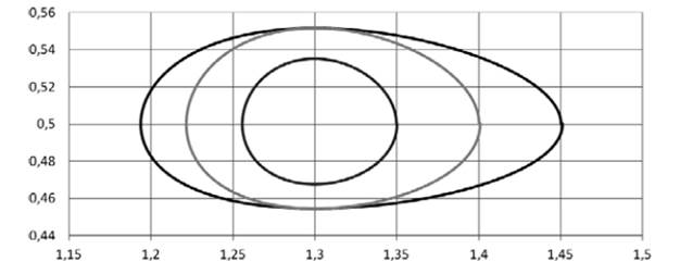
–ис. 4. ‘азовые портреты возможных циклов ондратьева типа Ђцентрї с одной и той же равновесной стационарной точкой х0= 1,3; у0= 0,5, но разными периодами и отклонени€ми от центра. ƒвижение по замкнутым орбитам идет против часовой стрелки. ѕериоды обращени€ по орбитам “= 50,1; 54,9; 60,6 лет
3. ѕЋјЌ —јћќ—“ќя“≈Ћ№Ќџ’ »——Ћ≈ƒќ¬јЌ»….
| Ётап | ¬ид работ | —роки | –езультат / ‘орма представлени€ результата |
| “еоретический | »зучение литературы по проблемной области исследовани€. »зучение экспериментальных данных. | 28 марта Ц 4 апрел€ | »ндивидуальный план работы. |
| ћоделирование | ќбобщение математической модели экономических циклов —.¬. ƒубовского | 4 апрел€ Ц 11 апрел€ | Ќаучна€ стать€ |
| јнализ моделей | ѕрименение экспериментальных данных к полученной обобщенной математической модели и анализ результатов. | 11 апрел€ Ц 16 ма€ | Ќаучна€ стать€, соответствующа€ плану исследований и теме диссертации. ѕредставление статьи на семинаре в Ќ»» прикладной математики и автоматизации г. Ќальчик |
| «авершающий | «авершение всех видов работы. —оставление и оформление отчета по практике. ѕодготовка отчетных документов (характеристик и пр.). | 16 ма€ Ц 29 ма€ | ќтчет по практике, ћагистерска€ диссертаци€, –укописи статей. |
4. –≈«”Ћ№“ј“џ —јћќ—“ќя“≈Ћ№Ќџ’ »——Ћ≈ƒќ¬јЌ»…
4.1 ќбобщенна€ модель ƒубовского, с учетом эффекта пам€ти в экономической системе.
ѕостановка задачи. ќбобщенна€ модель циклов ондратьева может быть представлена в виде:
 (1)
(1)
где  и
и  - производные дробных пор€дков
  в смысле √ерасимова- апуто;
 - гамма-функци€ Ёйлера;
 - эффективность новых технологий;
 - эффективность фондоотдачи;
 и
и  - равновесное стационарное решение системы (1);
 - норма накоплени€;
 - коэффициент, который определ€етс€ из статистики временного р€да;
  - внешнее воздействие на экономическую систему;
 - временна€ координата,
 - врем€ моделировани€ процесса;
 и
и  - начальные услови€, заданные константы.
«аметим, что нелинейна€ система (1) в случае значений параметров  и
и  переходит в модель ƒубовского [5]. ѕоэтому очевидно, что решение системы (1) будет обобщать решение модели ƒубовского.
–ешение нелинейной системы (1) будем искать с помощью численных методов Ц конечно разностных схем. –азобьем временной отрезок  на
на  равных частей, с шагом
  . јппроксимацию дробных производных в уравнении (1) проводим согласно работе [17]. “огда система (1) запишетс€ в конечно-разностной постановке в виде:
 (2)
(2)
«десь  .
.
–ешение (2) в случае, когда и  переходит в решение дл€ модели ƒубовского [4]. »сследуем решение (2) в зависимости от различных значений дробных параметров
  и
и  , а также построим фазовые траектории. ¬ этой работе мы не останавливаемс€ на вопросах устойчивости или сходимости €вной конечно разностной схемы (2).
–езультаты моделировани€.ѕараметры моделировани€ возьмем из работы [4]:  .
.

–ис. 5. –асчетна€ крива€ a и фазова€ траектори€ b в случае и
Ќа рис.5 приведен случай, который соответствует случаю из работы [4] при моделировании цикла ондратьева c периодом  . “ак же можно увидеть, что фазова€ траектори€ (рис. 1 b) имеет эллипсоидную замкнутую форму, равновесное состо€ние системы называетс€ центром. јмплитуда колебаний в этом случае посто€нна (рис. 1 a). Ќа рис. 2 приведен случай, когда ,
  и
и  , a остальные параметры остаютс€ без изменени€.

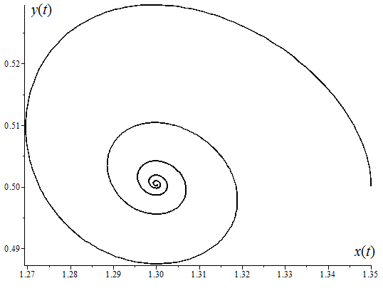
–ис. 6. –асчетна€ крива€ a и фазова€ траектори€ b в случае  и
и
»з рис. 6 a видно, что процесс колебаний €вл€етс€ затухающим, а фазова€ траектори€ рис. 6 b €вл€етс€ незамкнутой, положение равновеси€ системы называетс€ устойчивым фокусом. ¬ этом случае циклов не существует, однако, если ввести в рассмотрение функцию внешнего воздействи€  , которую можно интерпретировать как инвестиционные циклы, то приходим к следующему результату (рис. 3).

–ис. 7. –асчетна€ крива€ a и фазова€ траектори€ b в случае  и
и 
Ќа рис. 7 a видно, сначала амплитуда колебаний возрастает, а потом выходит на посто€нный режим, это видно на фазовой траектории рис.7 b, котора€ со временем выходит на посто€нный режим или предельный цикл, который можно использовать в исследовании циклов ондратьева.
4.2 јлгоритм реализаци€ моделировани€ в компьютерной среде Matlab
ѕример 1.
>restart;
>with(plots);
>n:=0.2;
>x0:= 1.3;
>y0:=0.5;
>x[0]:= 1.35;
>y[0]:=.5;
>lambda:= 2.25;
>T:= 50.1;
>N:= 1000;
>tau:=0.5;
>alpha:=0.8;
>beta:= 1;
>A:= tau^(-alpha)/GAMMA(2-alpha);
1.896275757
>B:= tau^(-beta)/GAMMA(2-beta);
2.000000000
>x[1]:= x[0]*(1-lambda*n*(x[0]-1)*(y[0]-y0)/A);
1.35
>y[1]:= y[0]*(1+(1-n)*n*(x[0]-x0)*y[0]/B);
0.5010000000
>x[2]:= x[1]*(1-lambda*n*(x[1]-1)*(y[1]-y0)/A);
1.349887872
>y[2]:= y[1]*(1+(1-n)*n*(x[1]-x0)*y[1]/B);
0.5020040040
>for j from 2 to N-1 do
x[j+1]:=x[j]*(1-lambda*n*(x[j]-1)*(y[j]-y0)/A)-(sum(((1+k)^(1-alpha)-k^(1-alpha))*(x[j-k+1]-x[j-k]), k = 1.. j-1));
y[j+1]:=y[j]*(1+(1-n)*n*(x[j]-x0)*y[j]/B)-(sum(((1+k)^(1-beta)-k^(1-beta))*(y[j-k+1]-y[j-k]), k = 1.. j-1))
end do;
>R:= seq([x[j], y[j]], j = 0.. N-1);
>pointplot([R], style = line);
ѕример 2.
>restart;
>with(plots);
>n:=0.2;
>x0:= 1.3;
>y0:=.5;
>x[0]:= 1.35;
>y[0]:=0.5;
>lambda:= 2.25;
>T:= 50;
>N:= 1250;
>tau:= 0.4e-1;
>alpha:=0.8;
>beta:=0.8;
>delta:=.5;
>omega:= 2;
>evalf(T/N);
>A:= tau^(-alpha)/GAMMA(2-alpha);
14.30307787
>B:= tau^(-beta)/GAMMA(2-beta);
14.30307787
>x[1]:= x[0]*(1-lambda*n*(x[0]-1)*(y[0]-y0)/A);
1.35
>y[1]:=y[0]*(1+(1-n)*n*(x[0]-x0)*y[0]/B)+evalf(delta*cos((0*omega)*tau));
1.000139830
>x[2]:= x[1]*(1-lambda*n*(x[1]-1)*(y[1]-y0)/A);
1.342565081
>y[2]:= y[1]*(1+(1-n)*n*(x[1]-x0)*y[1]/B)+evalf(delta*cos(omega*tau));
1.499100159
>for j from 2 to N-1 do
x[j+1]:=x[j]*(1-lambda*n*(x[j]-1)*(y[j]-y0)/A)-(sum(((1+k)^(1-alpha)-k^(1-alpha))*(x[j-k+1]-x[j-k]), k = 1.. j-1));
y[j+1]:=y[j]*(1+(1-n)*n*(x[j]-x0)*y[j]/B)-(sum(((1+k)^(1-beta)-k^(1-beta))*(y[j-k+1]-y[j-k]), k = 1.. j-1))+evalf(delta*cos(j*omega*tau))
end do;
>R:= seq([x[j], y[j]], j = 0.. N-1);
>RR:= seq([j*tau, x[j]], j = 0.. N-1);
>pointplot([RR], style = line);

>pointplot([R], style = line);

ѕример 3.
>restart;
>with(plots);
>n:=0.2;
>x0:= 1.3;
>y0:=0.5;
>x[0]:= 1.35;
>y[0]:=0.5;
>lambda:= 2.25;
>T:= 500;
>N:= 5000;
>tau:= 0.4e-1;
>alpha:= 1;
>beta:= 1;
>delta:= 0.1e-1;
>omega:= 1;
>evalf(T/N);
>A:= tau^(-alpha)/GAMMA(2-alpha);
25.00000000
>B:= tau^(-beta)/GAMMA(2-beta);
25.00000000
>x[1]:= x[0]*(1-lambda*n*(x[0]-1)*(y[0]-y0)/A);
1.35
>y[1]:= y[0]*(1+(1-n)*n*(x[0]-x0)*y[0]/B)+evalf(delta*cos((0*omega)*tau));
0.5100800000
>x[2]:= x[1]*(1-lambda*n*(x[1]-1)*(y[1]-y0)/A);
1.349914270
>y[2]:= y[1]*(1+(1-n)*n*(x[1]-x0)*y[1]/B)+evalf(delta*cos(omega*tau));
0.5201552594
>for j from 2 to N-1 do
x[j+1]:=x[j]*(1-lambda*n*(x[j]-1)*(y[j]-y0)/A)-(sum(((1+k)^(1-alpha)-k^(1-alpha))*(x[j-k+1]-x[j-k]), k = 1.. j-1));
y[j+1]:= y[j]*(1+(1-n)*n*(x[j]-x0)*y[j]/B)-(sum(((1+k)^(1-beta)-k^(1-beta))*(y[j-k+1]-y[j-k]), k = 1.. j-1))+evalf(delta*cos(j*omega*tau))
end do;
>R:= seq([x[j], y[j]], j = 0.. N-1);
>RR:= seq([j*tau, x[j]], j = 0.. N-1);
>pointplot([RR], style = line);

>pointplot([R], style = line);

«ј Ћё„≈Ќ»≈
¬ заключение необходимо отметить, что в разрезе проведенных исследований отраженных в индивидуальном плане практики, а также сбора информации дл€ написани€ выпускной магистерской диссертации, основна€ работа, проведенна€ в рамках преддипломной практики, на базе кафедры математики и физики была посв€щена моделированию динамики длинных волн Ќ.ƒ. ондратьева в экономической системе с учетом эффекта пам€ти, вы€влени€ общих и частных закономерностей, характера цикличности вышеуказанных волн, некоторых вопросов св€занных с особенност€ми затухани€ последних.
¬ рамках прохождени€ преддипломной практики были рассмотрены в комплексе различные научные подходы и экономико-математические модели диффузии инноваций и цикличности экономических кризисов.
¬ процессе изучени€ существующих математических моделей в предметной области была отобрана и обобщена модель —.¬. ƒубовского, поскольку данна€ модель соедин€ет экономический рост с научно-техническим прогрессом, то есть динамикой инноваций, что в свою очередь €вл€етс€ конечной целью проводимого исследовани€.
ѕолучено численное решение такой модели и построены фазовые траектории. ѕоказано, что введение производных дробного пор€дка приводит к затухающим процессам, однако если в системе существует внешнее периодическое воздействие, то система выходит на предельный цикл, который можно интерпретировать как цикл ондратьева.
¬ ходе прохождени€ преддипломной практики в целом было достигнуто решение задач поставленных научным руководителем, в частности:
- планирование научно-исследовательской работы;
- сбор материалов дл€ магистерской диссертации, обзор исследований в проблемной области;
- обоснование актуальности, новизны и практической значимости магистерской диссертации;
- проведение исследовательской работы согласно плану;
- апробаци€ результатов исследовани€ на региональных и всероссийских научных меропри€ти€х;
- подготовка научных статей;
- участие в работе научных коллективов;
- подготовка магистерской диссертации.
¬ представленном исследовании решены все поставленные задачи, результаты исследований имеют практическое значение, в целом однозначно интерпретируемы и соотнос€тс€ с тематикой магистерской диссертации.
—ѕ»—ќ Ћ»“≈–ј“”–џ
1. јбрамов, –. “еори€ длинных волн: исторический контекст и методологические проблемы // ¬опросы экономики. Ц 1992. Ц10. Ц — 17-19.
2. ƒубовский —.¬. ќбъект моделировани€ Ц цикл ондратьева // ћатематическое моделирование. 1995. “.7. Ц 6. Ц—. 65-74.
3. ƒубовский, —.¬. Ќаучно технический прогресс в глобальном моделировании. —истемные исследовани€. ≈жегодник. ћ.: Ќаука. Ц 1988. Ц —. 112-135.
4. ƒубовский, —.¬. Ёнергетика и распределение доходов в экономическом развитии. ћатематические модели. ћ.: ”–———. Ц 2004. Ц — 82-91.
5. ƒубовский —.¬. ћоделирование циклов ондратьева и прогнозирование кризисов. ¬ кн. ондратьевские волны. јспекты и перспективы / под. ред. јкаева ј.ј. ¬олгоград: ”читель, 2012. 179-188.
6. ƒубовский —. ¬. ѕрогнозирование катастроф (на примере циклов Ќ.ƒ. ондратьева) // ќбщественные науки и современность. Ц 1993. Ц 5. Ц —. 82-91.
7. ондратьев Ќ.ƒ., ќпарин ƒ.Ќ. Ѕольшие циклы конъюнктуры. ћ.: »нститут экономики, 1928. 287 с.
8. ћеньшиков, —.ћ., лименко, Ћ.ј. ƒлинные волны в экономике. ћ.: ћеждународные отношени€. Ц 1989. Ц —. 145-149.
9. ћакаров ƒ.¬. Ёкономико-математическое моделирование инновационных систем // ¬естник –ј”Ќ÷. ‘изико-математические науки. Ц 2014. Ц 1(8). Ц —. 66-70.
10. Ќахушев ј.ћ. ƒробное исчисление и его применение. ћ.: ‘изматлит, 2003. 272 с.
11. Ќахушева «.ј. ќб одной односекторной макроэкономической модели долгосрочного прогнозировани€ // ƒоклады јћјЌ. Ц 2012. “. 14. Ц 1. Ц —. 124-127.
12. ѕаровик –.». ћатематическое моделирование линейных эредитарных осцилл€торов. ѕетропавловск- амчатский: ам√” им. ¬итуса Ѕеринга, 2015. 178 с.
13. Boleantu M. Fractional dynamical systems and applications in economy // Differential Geometry - Dynamical Systems. Vol.10. 2008. pp. 62-70.
14. Krelle W. (Ed) The Future of the World Economy. Berlin. Springer-Verlad. Ц 1990. b.101.
15. Yiding Y., Lei H., Guanchun L. Modeling and application of new nonlinear fractional financial model // Journal of Applied Mathematics. 2013
16. Tejado I., Duarte V., Nuno V. Fractional Calculus in Economic Growth Modeling. The Portuguese case. Conference: 2014 International Conference on Fractional Differentiation and its Applications (FDA'14).
17. Mendes R.V. A fractional calculus interpretation of the fractional volatility model // Nonlinear Dyn. 2008.
18. Mensch. G. Stalemate in Technology. Innovations Overcome the Depression Cambrg. Ballinger Pub Co. 1979. 241 p.
19. Mesarovic M., Pestel E. (Eds) Multilevel Computer Model of World Development System. Laxenburg: IIASA. Ц 1974: b 60-65.
20. Zhenhua H., Xiaokang T. A new discrete economic model involving generalized fractal derivative // Advances in Difference Equations. 2015. V. 65. DOI 10.1186/s13662-015-0416-8.
21. Ўпилько я.≈., —оломко ј.ј., ѕаровик –.». ѕараметризаци€ уравнени€ —амуэльсона в модели Ёванса об установлении равновесно цены на рынке одного товара // ¬естник –ј”Ќ÷. ‘изико-математические науки. Ц 2012. Ц 2(5). Ц —. 33-36.
22. —амута ¬.¬., —трелова ¬.ј., ѕаровик –.». Ќелокальна€ модель неоклассического экономического роста —олоу // ¬естник –ј”Ќ÷. ‘изико-математические науки. Ц 2012. Ц 2(5). Ц —. 37-41.
ѕ–»Ћќ∆≈Ќ»≈ ј
—ѕ»—ќ Ќј”„Ќџ’ —“ј“≈…
| є п/п | Ќаименование работы, ее вид | ‘орма работы | ¬ыходные данные | ќбъем в с. | —оавторы | |||||
| ƒинамическа€ математическа€ модель экономических кризисов с учетом инвестиционного цикла (стать€ –»Ќ÷) | ѕечатна€ | “еори€ и практика современных гуманитарных и естественных наук. ¬ыпуск 6: сборник научных статей ежегодной межрегиональной научно-практической конференции, ѕетропавловск- амчатский, 03-06 феврал€ 2016 г. / отв. ред. ¬. ¬. ƒавыдов, ќ. ¬. Ўереметьева; ам√” им. ¬итуса Ѕеринга. Ц ѕетропавловск- амчатский: ам√” им. ¬итуса Ѕеринга, 2016. Ц —. 38-40. | 6 с | ѕаровик –.». | ||||||
|
|
|
|
|
ƒата добавлени€: 2017-02-25; ћы поможем в написании ваших работ!; просмотров: 303 | Ќарушение авторских прав
Ћучшие изречени€:
 | 1574 -
√ен: 0.495 с.