


Now letТs look at some of the rules for creating formulas: The operators that you need to know are
+ addition
- subtraction
* multiplication
/ division
^ exponentiation (Уto the power of)
& to join two text strings together These operations are evaluated in a particular order of precedence by Excel:
Х Operations inside brackets are calculated first
Х Exponentiation is calculated second.
Х Multiplication and division are calculated third.
Х Addition and subtraction are calculated fourth.
Х When you have several items at the same level of precedence, they are calculated from left to right.
LetТs look at some examples:
= 10 + 5 * 3 - 7 (result: 10 + 15 - 7 = 18)
= (10 + 5) * 3 - 7 (result: 15 * 3 - 7 = 38)
= (10 + 5) * (3 - 7) (result: 15 * -4 = -60)
If youТre not sure how a formula will be evaluated - use brackets!
Calculation operators in formulas
Operators specify the type of calculation that you want to perform on the elements of a formula. Microsoft Excel includes four different types of calculation operators: arithmetic, comparison, text, and reference.
Х Arithmetic operators perform basic mathematical operations such as addition, subtraction, or
multiplication; combine numbers; and produce numeric results.
| Arithmetic operator | Meaning | Example |
| + (plus sign) | Addition | 3+3 |
| - (minus sign) | Subtraction | 3-1 |
| Negation | -1 | |
| * (asterisk) | Multiplication | 3*3 |
| / (forward slash) | Division | 3/3 |
| % (percent sign) | Percent | 20% |
| ^ (caret) | Exponentiation | 3^2 (the same as 3*3) |
Х Comparison operators compare two values and then produce the logical value TRUE or FALSE.
| Comparison operator | Meaning | Example |
| = (equal sign) | Equal to | A1=B1 |
| > (greater than sign) | Greater than | A1>B1 |
| < (less than sign) | Less than | A1>B1 |
| >= (greater than or equal to sign) | Greater than or equal to | A1 >=B1 |
| <= (less than or equal to sign) | Less than or equal to | A1<=B1 |
| <> (not equal to sign) | Not equal to | AK>B1 |
Х The text operator "&" combines one or more text values to produce a single piece of text.
| Text operator | Meaning | Example |
| & (ampersand) | Connects, or concatenates, two values to produce one continuous text value | "North" & "wind" produce "Northwind" |
Х Reference operators combine ranges of cells for calculations.
| Reference operator | Meaning | Example |
| : (colon) | Range operator, which produces one reference to all the cells between two references, including the two references | B5:B15 |
| ,(comma) | Union operator, which combines multiple references into one reference | SUM(B5:B15,D5:D15) |
| (single space) | Intersection operator, which produces one reference to cells common to two references | SUM(B5:B15A7:D7) In this example, cell B7 is common to |
Summary functions for data analysis
| Function | Summarizes |
| Sum | The sum of the values. This is the default function for numeric source data. |
| Count | The number of items. The Count summary function works the same as the COUNTA worksheet function. Count is the default function for source data other than numbers. |
| Average | The average of the values. |
| Max | The largest value. |
| Min | The smallest value. |
| Product | The product of the values. |
| Count Nums | The number of rows that contain numeric data. |
| The Count Nums summary function works the same as the COUNT worksheet function. | |
| StdDev | An estimate of the standard deviation of a population, where the sample is all of the data to be summarized. |
| StdDevp | The standard deviation of a population, where the population is all of the data to be summarized. |
| Var | An estimate of the variance of a population, where the sample is all of the data to be summarized. |
| Varp | The variance of a population, where the population is all of the data to be summarized |
|
|
|
Relative cell referencing
Remember in the pricing example above, how you just had to copy the formulas in row 2 and the remaining values were automatically calculated?
Look again in the formula bar of that screenshot. Although the formula that you copied from cell G2 was У=F2 * 95%Ф, the formula in cell G5 reads У=F5 * 95%Ф. The original reference to row 2 in the formula has changed to a reference to row 5. This is called relative addressing, and itТs an important concept.
Relative addressing is what Excel uses by default. This means that when you copy or move a formula to a new location in a worksheet (or even to another workbook), Excel automatically adjusts the cell references in the copied formula to be consistent with the original formula. If the original formula referenced a value five columns to the left and two rows down, then the copied formula will do the same.
Does this concept make sense? If not, then give it some careful thought, because itТs important that you understand it.
Absolute cell referencing
Now weТre going to improve the structure and usability of our pricing model. After all, thereТs no guarantee that your markup will always be 25% - in these tough economic times you may need to reduce it to remain competitive. And what if the VAT rate changes? Or maybe you decide to increase the discount to encourage customers to pay promptly?
The following example shows you how to construct the worksheet so that it allows for future changes in the business.
Here IТve made life a lot easier for myself by showing the markup, the VAT rate, and the customer discount, in cells A1 to B3. I no longer have to remember what values I used in my formulas - I can just look at the top of the worksheet.
Now my formulas need to change, so that they refer to the values in cells B1 to B3 instead of physically typing the actual percentages in each formula.
Х The formula in cell C5 will become У=B5 * B1Ф, instead of the previous У=B5 * 25%Ф. This multiplies the value in cell B5 (cost price) by the value in cell B1 (markup rate), and displays the result in cell C5 (markup).
Х The formula in cell E5 will become contains У=D5 * B2Ф, instead of the previous У=D5 * 14%Ф. This multiplies the value in cell D5 (retail price) by the value in cell B2 (VAT rate), and displays the result in cell E5 (selling price).
|
|
|
Check that you follow the logic so far. If not, please go through it again.
BUTЕ Stop right here! Do you see the problem ahead?
When I copy my new formulas from row 5 into rows 6 to 8, Excel is going to use relative addressing. The formula in cell C5 refers to cell B1 (the markup rate). When I copy the formula to the next row, it will want to refer to cell B2 (the VAT rate), instead of cell B1 (the markup rate). By the time IТve finished copying, my spreadsheet will look like this:

Clearly something is very wrong!
Relative addressing makes working with formulas really easy, but sometimes you donТt want the referencing in the formula to change as the formula is copied. Then you need to use absolute addressing. Absolute addressing fixes a cell reference so that regardless of where the formula is copied to, it will always reference the same original cell. This feature takes the versatility of formulas to the next level!
To use absolute addressing in a formula, all you need do is to click on the cell reference that you want to remain fixed, and then press the [F4] key. Take for example the formula in cell C5:
Using relative addressing, the formula looked like this: = B5 * B1
1. Double click on cell C5 to enter edit mode.
2. In the formula bar, click on the cell reference УB1Ф and press [F4] on the keyboard.
3. The formula changes to: =B5 * $B$1. Note that cell reference B5 must retain its relative addressing, since you want to multiply each different cost price by the same fixed markup rate.
4. Press [ENTER] to accept the change.
| Instead of using the [F4] key to make a cell reference absolute, you can simply type the dollar signs if you prefer to do so. |
Instead of using the [F4] key to make a cell reference absolute, you can simply type the dollar signs if you prefer to do so.
Once all the formulas in row 5 have been corrected to use absolute referencing, you can copy them into rows 6 to 8. The following screenshot shows the result Ц now it all works perfectly!

Any future changes to the markup rate, VAT rate or discount rate need only be entered once in cells B1 to B3 (where they are clearly visible), and the calculated values from row 5 downwards will automatically be updated!
Functions
Excel provides a wide range of built-in functions that can be included in your formulas to save you the effort of having to specify detailed calculations step-by-step. Each function is referred to by a specific name, which acts as a kind of shorthand for the underlying calculation. Because a function is used inside a formula, youТll still need to start off with an equals sign to show Excel that a calculation is required.
Using AutoSum
 Because addition is the most frequently used Excel function, a shortcut has been provided to quickly add a set of numbers:
1. Select the cell where you want the total to appear.
2. Click on the Sum button on the Home ribbon.
3. Check that the correct set of numbers has been selected (indicated by a dotted line). If not, then drag to select a different set of numbers.
4. Press [ENTER] and the total will be calculated.
Basic functions
Some of the most commonly used functions include:
SUM() to calculate the total of a set of numbers
AVERAGE() to calculate the average of a set of numbers
MAX() to calculate the maximum value within a set of numbers
MIN() to calculate the minimum value within a set of numbers
ROUND() to round a set a values to a specified number of decimal places
TODAY () to show the current date
IF() to calculate a result depending on one or more conditions
So how do you use a function?
A function makes use of values or cell references, just like a simple formula does. The numbers or cell references that it needs for its calculations are placed in brackets after the name of the function.
To give a simple illustration:
|
|
|
| The formula: | is equivalent to the function: |
| = 12 + 195 + 67 Ц 43 | = SUM(12, 195, 67, -43) |
| = (B3 + B4 + B5 + B6) | =SUM(B3:B6) |
| = (B3 + B4 + B5 + B6)/4 | = AVERAGE (B3:B6) |
 Several popular functions are available to you directly from the Home ribbon.
1. Select the cell where you want the result of the calculation to be displayed.
2. Click the drop-down arrow next to the Sum button.
3. Click on the function that you want.
4. Confirm the range of cells that the function should use in its calculation. (Excel will try to guess this for you. If you donТt like what it shows inside the dotted line, then click and drag to make your own selection.)
5. Press [ENTER]. The result of the calculation will be shown in the active cell.
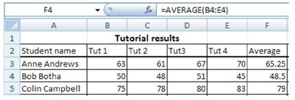
As an example, to calculate the average for the following set of tutorial results, you would:
1. Click on cell F3 to make it active.
2. Click on the arrow next to the Sum button, and select Average.
3. Press [ENTER] to accept the range of cells that is suggested (B3:E3).
ThatТs it! You can now copy the formula in cell F3 down to cells F4 and F5 Ц using relative addressing because you want a different set of tutorial marks to be used for each student.
If you want to use a function that isnТt directly available from the drop-down list, then you can click on More Functions to open the Insert Function dialog box. Another way to open this dialog box is to click the Insert Function icon on the immediate left of the formula bar.
The Insert Function dialog box displays a list of functions within a selected function category. If you select 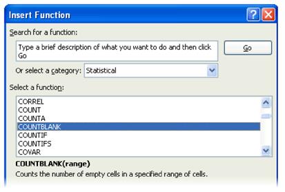 a function it will briefly describe the purpose and structure of the function.
When you click the OK button at the bottom of the window, youТll be taken to a second dialogue box that helps you to select the function arguments (usually the range of cells that the function should use).
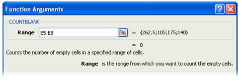
Some functions use more than one argument. For example, the ROUND() function needs to know not only which cells to use, but also how many decimal places those cells should be rounded to. So the expression =ROUND(G5:G8, 0) will round the values in cells G5 to G8 to the nearest whole number (i.e. no decimal places).
| Note that the ROUND() function actually changes the value that is stored in your worksheet, based on the arguments youТve provided. Formatting options such as Currency, or Increase / Decrease Decimal, simply change the appearance of a number, but all its decimal places are still kept, and displayed in the formula bar. |
The IF() function
The IF() function is getting a section all of its own, because for many people itТs not as intuitive to understand as the common maths and stats functions.
The IF() function checks for a specific condition. If the condition is met, then one action is taken; if the condition is not met, then a different action is taken. For example, you may be reviewing a set of tutorial marks. If a studentТs average mark is below 50, then the cell value should be FAIL; so the condition you are checking is whether or not the average result is below 50. If this condition is not met (that is, the average result is 50 or more), then the cell value should be PASS.
LetТs see this in action:
The structure of an IF() function is:
=IF (condition, result if true, result if false)
Using English to describe our example as an IF statement: IF the average mark is less than 50, then display the word УFAILФ, else display the word УPASSФ.
Now for a real worksheet example. Look at the formula bar in the screenshot below:
Do you follow how the formula in cell G4 was constructed? Because the average mark is stored in cell F4, we need to check whether the value in F4 is less than 50. If it is, then the active cell (G4) must display the word УFailФ. If the value in F4 is not less than 50, then the active cell must display the word УPassФ. ThatТs not really so complicated, is it?
|
|
|
Nested functions
Take a deep breath and donТt panic! I just want to show you that if you need to, you can include one function inside another.
In the example above, we first worked out the Average mark, and then the Pass/Fail outcome. But we could have done it all in a single step, by using the following formula in row 3:
=IF(AVERAGE(B3:E3) < 50, УFAILФ, УPASSФ)
In this IF statement, IТve nested one function inside another. The reference to cell F4 has been replaced with a function that calculates the average tutorial mark, and then checks it against the same condition as before (У< 50Ф), with the same possible outcomes. Doing it this way, you wouldnТt need column F in the worksheet at all.
Of course, in real life youТd expect to get students coming to query their Pass/Fail status, and would probably want to keep the Average column to explain the outcome thatТs been allocated to them. So the first example using a separate Average and Outcome is not only simpler, itТs also more practical!
Printing
By default, Excel prints all the data on the current worksheet. If your worksheet extends over several pages, itТs worth making sure that the printed copy will be easily readable. Here are a few tips.
Print preview
Start by using Print Preview to see what your data will look like when itТs printed.
1. Click the Office button, select Print and then Print Preview. The Print Preview icon
shows a dog-eared page with a magnifying glass.

 2. The display will change to Print Preview mode. You see the document exactly as it
will look when printed.
3. The Show Margins option allows you to not only adjust your page
margins by dragging them, but also to drag the column and row
boundaries to make them narrower or wider.
4. Now is the time to consider whether the column and row labels are easily visible,
whether page breaks are in appropriate places, and whether you need to include
page numbers. The following section tells you how to do all these.
5. To close Print Preview, click the Close Print Preview button on the right of the
ribbon.
Preparing to print
Your best option is to use the Page Layout ribbon for this. (Some of the same options are available from inside Print Preview, but many of them arenТt.)

Х Use the Orientation button to swap between portrait and landscape mode.
Х Use the Print Area button to select a subset of your data for printing. (The data that you want included in the print area should be selected before you click this icon.)
Х Use the Breaks button to insert a page break immediately above the currently
active cell, or to remove previously specified page breaks.
The Print Titles button takes you to the Page Setup dialogue box, which has four tabs that allow you to do a whole lot more than printing titles.

The Page tab is used to set orientation and scaling.
The Margins tab is used to adjust page margins.
The Header/Footer tab allows you to enter a header or footer to be repeated on every page. This is where you would include page numbers.
The Sheet tab lets you specify rows that are to be repeated at the top of each sheet (such as column headings), and columns to be repeated at the left of each sheet (such as student names). You can also adjust the print area under this tab.

| If you donТt know the cell ranges to be included in the print area, or to be repeated on each page, then you can either drag the dialog box to a different area of the screen, or else click the collapse dialog button on the right of the data entry field to allow you to navigate within the worksheet. |
Printing a worksheet
YouТve previewed your worksheet one last time, and youТre happy with the way it looks - now itТs time to finally print it!
1. Click the Office button and select the Print command.
2. The Print dialog box will appear.

3. If you have more than one printer to choose from, they will be available in the Printer area. Click the drop-down arrow next to the Name field to select your preferred printer.
4. Would you like to print selected pages only? Find the Page Range area, and type the page numbers that youТd like printed in the Pages field.
5. If youТd like to print the entire workbook, rather than just the active sheet, you can specify this in the Print What area of the dialog box.
|
|
|
6. If youТd like more than one copy of the worksheet, then enter the required number of copies in the Number of Copies field.
7. Click OK when youТre satisfied with your settings. The specified worksheet pages will be sent to the printer.
Charts
A picture is worth a thousand words! Often itТs much easier to understand data when itТs presented graphically, and Excel provides the perfect tools to do this!
ItТs worth starting with a quick outline of different data types and charts:
Categorical data items belong to separate conceptual categories such as knives, forks and spoons; or males and females. They donТt have inherent numerical values, and it doesnТt make sense to do calculations such as finding an average category. A pie chart or column chart is most suitable for categorical data.
Discrete data items have numerical values associated with them, but only whole values; for example, the number of TV sets in a household. Again, average values donТt make much sense. Discrete data is often grouped in categories (Уless than threeФ, Уfour or moreФ) and treated as categorical data.
Continuous data refers to numerical values that have an infinite number of possible values, limited only by the form of measurement used. Examples are rainfall, temperature, time. Where discrete data has a very large number of possible values, it may also be treated as continuous. Continuous data is well suited to line graphs, which are very useful for illustrating trends.
Of course, Excel offers you many more chart types than just these three. Do remember that itТs best to select a chart type based on what youТre trying to communicate.
Excel Help  has a lot of useful information. Look under Charts in the Table of Contents. has a lot of useful information. Look under Charts in the Table of Contents.
|
Creating a chart
ItТs very easy to create a basic chart in Excel:
1. Select the data that you want to include in the chart (together with column headings if you have them).
2. Find the Charts category on the Insert ribbon, and select your preferred chart type.

3. ThatТs it! The chart appears in the current window. Move the cursor over the Chart
Area to drag it to a new position.

Modifying a chart
When you click on a chart, a Chart Tools section appears on your Ribbon, with Design, Layout and Format tabs.
Х Use the Design tab to quickly change the chart type, or to swap data rows and
columns.

In this example, IТve changed the previous chart type to Column, and swapped rows and columns. All it took was two mouse clicks!

Х Use the Layout tab to add a title, and to provide axis and data labels.
Х Use the Format tab to add border and fill effects.

