


Click the °∞Display Serial Number°± as  , to display the pixel°ѓs processing sequence serial number.
Figure 3-79
Display jumper
Click the °∞Display Jumper°± button as  , to display the jumper between pixels.
Figure 3-80
Display processing direction
Click the °∞Display Direction°± button as  and the pixel processing direction will be shown.
Figure 3-81
Display the starting point
Click the °∞Display the Starting Point°± button as  and the starting point of processing of the pixel will be shown.
Figure 3-82
Chapter IV Output Processing
Layer Parameters
Layer parameters are relevant to colors. The same kind of colors uses the same layer parameter. There is a list of layer parameters at the bottom of the °∞Working°± page in the dialog box toolbar in the right part of main interface of the software. See Figure 4-1.
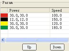
Figure 4-1
As shown in Figure 4-1, the layers from top to bottom in the list indicates the sequence of processing. Red layer pixels are the first to be processed, followed by black layer, yellow layer and green layer successively. After selecting a layer, it is allowed to change the processing sequence by clicking the [Move up] or [Move down] buttons.
Pitch on a certain layer and double click the mouse, to open the parameter setting dialog box, as shown in Figure 4-2.
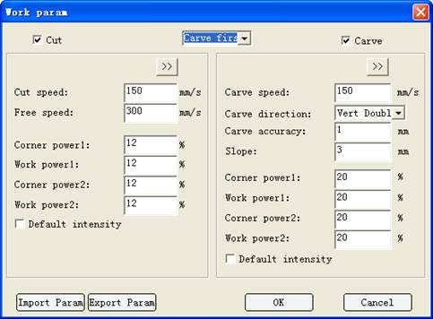
Figure 4-2
Set parameters for the current layer.
Cutting and carving priority setting
If a layer needs to go through cutting and carving, it is allowed to set the sequence of them two. Click the list box as shown in Figure 4-3 to set their priority.

Figure 4-3
Cutting parameters
When setting cutting parameters as shown in Figure 4-4, it needs to click the [Cut] option as  first.
The parameter of Light Intensity 1 is corresponding to the first laser head and that of Light Intensity 2 to the second one.
[Cutting Speed]: refers to the movement speed of laser heads during bright dipping processing. When it is set as 0, the default processing speed of the control card will be used.
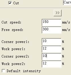
Figure 4-4
[Traveling Speed]: the movement speed of laser head under non-bright dipping non-processing state. When it is set as 0, the default traveling speed of the control card will be used.
[Turning Light Intensity]: the light intensity sent out by laser at corners.
[Working Light Intensity]: the light intensity sent out by laser when reaching the cutting speed.
[Default Light Intensity]: when default light intensity is selected, default light intensity parameter set on the control card will be used.
[>>]: click the °∞extend°± button and a dialog box for setting of the cutting extension function will pop up. See Figure 4-5.
[Blow]: it defines whether the draught fan is working or not when the device is in operation; if [Blow] and [Auto Control] are selected, only when laser sends out light, will the device °∞blow°±; if [Blow] is selected but not [Auto Control], the device will °∞blow°± in the whole process.
|
|
|
[Start-up Delay]: it defines the time that a laser waits for light dipping in situ at the beginning of a pixel.
[Finish Delay]: it defines the time that a laser waits for light dipping in situ at the end of a pixel.
[Dot]: it allows users to make smooth line graphs work in discontinuous dot mode.
[Interval]: it refers to the distance between dots.
[Time]: it refers to the time of bright dipping in situ when doting a point.
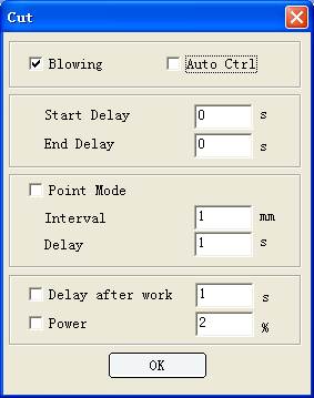
Figure 4-5
[Post-processing Delay]: it refers to the retention time after layer processing finishes.
[Light Intensity]: it refers to the light intensity kept by the laser tube during post-processing delay.
Carving parameters
Before setting carving parameters, please select the °∞Carve°± button as  first. See Figure 4-6£Ї
[Carving Speed]: it refers to the working speed during normal bright dipping.
[Carving Mode]: it refers to the working mode during device bright dipping, which is divided into °∞horizontal & unidirectional°±, °∞horizontal & bidirectional°±, °∞vertical & unidirectional°± and °∞vertical & bidirectional°±.
[Carving Precision]: it refers to the distance between two neighboring bright dipping lines.
[Slope]: set the slope length for slope carving. Turning light intensity determines top depth. The stronger the turning light intensity is, the deeper the top will be; working light intensity determines graph depth. The stronger the light intensity is, the deeper the graph will be; slope distance determines the distance from the slope top to the bottom. The larger the distance is, the gentler the slope will be.
[Turning Light Intensity]: it refers to the laser light intensity in slope carving.
[Working Light Intensity]: it refers to the light intensity during bright dipping operation or the light intensity used at the deepest point of the graph in slope carving.
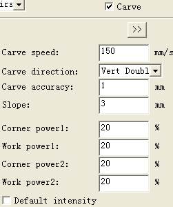
Figure 4-6
[>>]: click the °∞Extend°± button and the dialog box for extended carving functions will pop up. Click to open it, as shown in Figure 4-7.
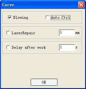
Figure 4-7
[Blow]: it defines whether the draught fan is working or not when the device is in operation; if [Blow] and [Auto Control] are selected, only when laser sends out light, will the device °∞blow°±; if [Blow] is selected but not [Auto Control], the device will °∞blow°± in the whole process.
[Light Spot Compensation]: if the laser light spot compensated is too large, the size of graph will become smaller or blur. After setting the diameter of the light spot (in mm), select [Light Spot Compensation] to enable the function.
[Post-processing Delay]: it refers to the retention time after layer processing finishes. After setting the delay time (in second), select [Post-processing Delay] to enable the function.
Online Control
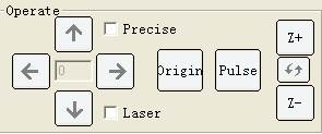
Figure 4-8
By making online control, independent software can control machine motion. Simple processing does not need drawing and can be finished by online control, such as single line cutting and rectangle cutting. Rising and falling of the lifting axis and feeding of the feed axis can be controlled online by independent software.
Control mode
A) Network
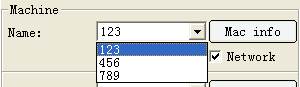
Figure 4-9
The procedures are as following.
|
|
|
1£© Connect two ends of the network cable to PC and the machine respectively.
2£© Select the [Working] page on the right side of the software interface.
3£© Find the machine to be connected in [Equipment Name] (if there is no machine name, make machine management as introduced in 2.1) and select it.
4£© Select [Start the Network].
5£© Finish.
B£©USB

Figure 4-10
The procedures are as following.
1£© Connect two ends of the USB line to PC and the machine respectively.
2£© Select the [Working] page on the right side of the software interface.
3£© Click [Search] to search the port number.
4£© Click the pull-down list of [Port Number] to select the port.
5£© Finish.
Movement
After clicking the  button, the laser head does not move in horizontal direction, but moves upwards for a certain distance in vertical direction. If the moving direction is found to be reversed, it is necessary to set the button polarity of the Y-axis in machine parameters. In case of long-term pressing, the laser head will keep moving until the button is released.
After clicking the  button, the laser head does not move in horizontal direction, but moves downwards for a certain distance in vertical direction. If the moving direction is found to be reversed, it is necessary to set the button polarity of the Y-axis in machine parameters. In case of long-term pressing, the laser head will keep moving until the button is released.
After clicking the  button, the laser head does not move in vertical direction, but moves leftwards for a certain distance in horizontal direction. If the moving direction is found to be reversed, it is necessary to set the button polarity of the X-axis in the machine parameters. In case of long-term pressing, the laser head will keep moving until the button is released.
After clicking the  button, the laser head does not move in vertical direction, but moves rightwards for a certain distance in horizontal direction. If the moving direction is found to be reversed, it is necessary to set the button polarity of the X-axis in the machine parameters. In case of long-term pressing, the laser head will keep moving until the button is released.
Click  to set the point where the laser head currently locates as the °∞locating point°±,
Clicking  , the laser head will emit light in the original position without moving until releasing the button.
Click the control button in the up and down directions of the axis cyclic switching button  to cyclically switch among [Z-axis] °ъ [U-axis] °ъ [V-axis].
Click  to make the Z-axis move in positive direction, and if the moving direction is reversed, set the button polarity of the Z-axis in machine parameters.
Click  to make the Z-axis move in negative direction, and if the moving direction is reversed, set the button polarity of the Z-axis in machine parameters.
Click  to make the U-axis move in positive direction, and if the moving direction is reversed, set the button polarity of the U-axis in machine parameters.
Click  to make the U-axis move in negative direction, and if the moving direction is reversed, set the button polarity of the U-axis in machine parameters.
Click  to make the V-axis move in positive direction, and if the moving direction is reversed, set the button polarity of the V-axis in machine parameters.
Click  to make the V-axis move in negative direction, and if the moving direction is reversed, set the button polarity of the V-axis in machine parameters.
[Bright Dipping]: after being checked, it will always emit light no matter which direction it moves to, including [Up], [Down], [Left] and [Right].
[Precise Movement]: After being checked, it can input distance in the middle edit box of the up, down, left and right buttons, and after clicking direction buttons, the laser head will move from the current position for the input distance. If the input value is positive, the moving direction complies with the button direction; while if negative, the direction will be reversed.
|
|
|
Rout Optimization
Before downloading graphs, in order to process in the specific rout and increase processing speed, please optimize its rout; select [Download], check [Rout Optimizing] and click the button of [<<] to enter the rout setting dialog box:
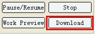
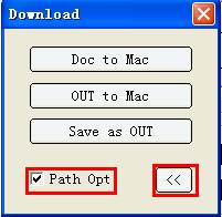
Figure 4-11
After clicking the  button, the following interface appears:
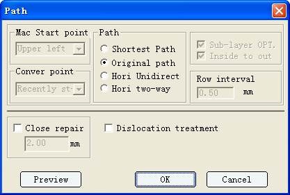
Figure 4-12
Optimization type
User-defined rout optimization includes: shortest rout, horizontal one-way and horizontal two-way.
[Shortest Rout]: for graphs in non-array model, take the shortest rout of laser head°ѓs moving distance as the processing rout.
[Horizontal One-way]: for array graphs or regularly arrayed graphs, process line by line from top to bottom and from left to right, with the processing direction of closed curves in the same line being the same, anticlockwise or clockwise.
[Horizontal Two-way]: for array graph or regularly arrayed graphs, process line by line from top to button in S shape, with the processing direction of closed curves in the same line being the same, anticlockwise or clockwise. (e.g.: process from left to right for one line, and process from right to left for the following line.)
[Original Route]: no any optimization is done.
Additional parameter
[Processing Starting Point]: indicates that it starts to work from certain position of the graph (top left, top right, low left, low right, etc.).
[Optimize by Layers]: whether to optimize in layers or it is allowed to optimize across layers.
[Inside Out]: Firstly process the smaller graphs inside, and then the larger graphs outside.
[Nearest Starting Point]: modify the starting point of the original graph to make the empty moving distance shortest.
[Smooth Starting Point]: modify the starting point of the original graph to make the speed varies gently.
[Original Starting Point]: do not modify the starting point of the original graph (which is suitable to manually assign starting point or graphs with lead).
Malposition disposal
In case of different processed component sizes or seal malposition making it impossible to be cut off, check this option for solution. Check the check box as  of °∞Malposition Disposal°±, and it will always dispose the malposition no matter whether or not route optimization has been done.
Closure compensation
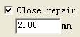
Figure 4-13
During material cutting, the potential inconformity between the minimum light intensity of laser tube and the material photonasty and processing speed may lead that though the sealing position of closed graph can emit light, it can not be cut off, for which, the function of °∞Closure Compensation°± is provides in the software to over cut a certain distance to solve this problem. The distance value should be set as actually needed. After checking the check box as  of °∞Closure Compensation°±, it will always conduct closure compensation no matter whether or not route optimization has been conducted.
Manual sorting
Click the menu of [Function], and click [Manual Sorting] as shown in the following:
Figure 4-14
The following sorting interface appears in the toolbar of the dialog box on the right of the main interface:
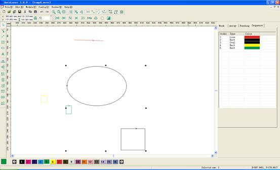
Figure 4-15
In the pixel list, left click one of the pixels and remain; drag the mouse to the target position and release it, when the position shown in the right list will be the processing sequence of the pixels in current file.
Note: After manual sorting, it does not need to optimize route, otherwise it will cause inconformity between the processing sequence and the setting.
|
|
|
Working Pretreatment
Border preview
Before processing, it is allowed to firstly select °∞Border Away°± to check the breadth of the processing graph and the °∞Working°± page of the toolbar in the right dialog box of the main interface of the software is as shown in the following
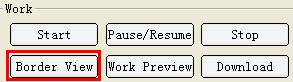
Figure 4-16
[Border Away]: Click the  button, and the interface appears as follows:
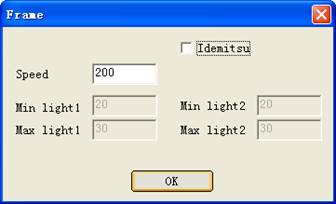
Figure 4-17
If there is graph file at present, the machine takes the current locating point as the benchmark point. Operate along minimum enclosing rectangle of the current file, and execute during the motion according to the defined speed and light intensity to see whether light comes out.
Working preview
The °∞Working°± page of the toolbar of the right dialog box of the main interface of the software is as shown in the following figure:
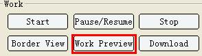
Figure 4-18
[Working Preview]: it is allowed to conduct simulating processing to the working file downloaded to the machine, check the process route, etc.
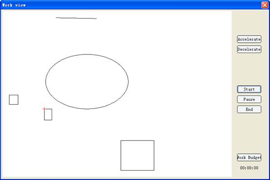
Figure 4-19
[Start]: start simulating processing.
[Suspend]: suspend simulating processing.
[Stop]: stop simulating processing.
[Accelerate]: accelerate simulating processing speed.
[Slowdown]: slowdown the simulating processing.
[Man-hour Prediction]: asset the processing time of the file.
Output Processing
After setting the processing parameters, it is allowed to execute output processing as shown in Figure 4-20:
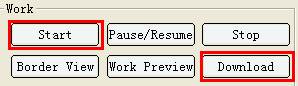
Figure 4-20
[Start]: download current file to the control card, and directly start to work, regarding current file as the processing file.
[Suspend/Continue]: continue or suspend the processing.
[Stop]: stop the processing.
[Download]: click the download button to pop up the download dialog box as shown in Figure 4-21:
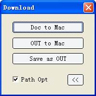
Figure 4-21
[Download]: download current file to the control card (it will not work directly).
[Offline File Output]: download the previously saved file to the control card (it will not work directly).
[Save Offline File]: save the current file in the processing format (out file) to the designated position of the computer.

